

3.2 One-Body Completeness Relation
95
u
(s)
n (r ) is finite and is the same when R (s) → +∞. This arises because the nodes of
u(k = 0, r ) are in finite number, u (s) (k = 0, r ) ∝ u(k = 0, r ) if 0 ≤ r ≤ R (s)
and u (s) (k = 0, r ) ∝ u (k = 0, R (s) )(r − R (s) ) + u(k = 0, R (s) ) if r ≥ R (s) (see
Eq. (2.5)). Indeed, if u(k = 0, r ) is not a bound state, |u(k = 0, r )| → +∞, so
that, for R (s) sufficiently large, |u (s) (k = 0, r )| → +∞ for r → +∞ and all
zeros of u(k = 0, r ) and u (s) (k = 0, r ) can be situated in [0 : R (s) ]. Alternatively,
if u(k = 0, r ) is a bound state, for R (s) sufficiently large, u (s) (k = 0, r ) possesses
a single zero for r > R (s) , so that the number of zeros of u(k = 0, r ) (including
the one at infinity) and u (s) (k = 0, r ) are the same. Therefore, u
(s)
n (r ) and u n (r )
are normalized bound states of n nodes which solve Eq. (2.2), respectively, for 0 ≤
r ≤ R (s) and for all radii. Consequently, u
(s)
n (r ) → u n (r ) when R (s) → +∞
by unicity of u n (r ) (see Exercise I of Chap. 2). Therefore, δ b (R (s) ) vanishes when
R (s) → +∞.
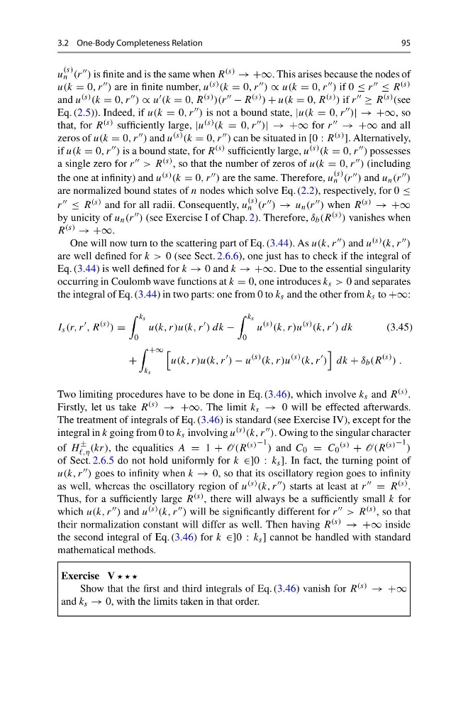
One will now turn to the scattering part of Eq. (3.44). As u(k, r ) and u (s) (k, r )
are well defined for k > 0 (see Sect. 2.6.6), one just has to check if the integral of
Eq. (3.44) is well defined for k → 0 and k → +∞. Due to the essential singularity
occurring in Coulomb wave functions at k = 0, one introduces k s > 0 and separates
the integral of Eq. (3.44) in two parts: one from 0 to k s and the other from k s to +∞:
I s (r, r
, R
(s) ) =
k s
0
u(k, r)u(k, r
) dk −
k s
0
u
(s) (k, r)u
(s) (k, r
) dk
(3.45)
+
+∞
k s
u(k, r)u(k, r
) − u
(s) (k, r)u
(s) (k, r
)
dk + δ b (R
(s) ) .
Two limiting procedures have to be done in Eq. (3.46), which involve k s and R (s) .
Firstly, let us take R (s) → +∞. The limit k s → 0 will be effected afterwards.
The treatment of integrals of Eq. (3.46) is standard (see Exercise IV), except for the
integral in k going from 0 to k s involving u (s) (k, r ). Owing to the singular character
of H
±
,η (kr), the equalities A = 1 + O(R (s) −1 ) and C 0 = C 0
(s) + O(R (s) −1 )
of Sect. 2.6.5 do not hold uniformly for k ∈]0 : k s ]. In fact, the turning point of
u(k, r ) goes to infinity when k → 0, so that its oscillatory region goes to infinity
as well, whereas the oscillatory region of u (s) (k, r ) starts at least at r = R (s) .
Thus, for a sufficiently large R (s) , there will always be a sufficiently small k for
which u(k, r ) and u (s) (k, r ) will be significantly different for r > R (s) , so that
their normalization constant will differ as well. Then having R (s) → +∞ inside
the second integral of Eq. (3.46) for k ∈]0 : k s ] cannot be handled with standard
mathematical methods.
Exercise V
Show that the first and third integrals of Eq. (3.46) vanish for R (s) → +∞
and k s → 0, with the limits taken in that order.
95
u
(s)
n (r ) is finite and is the same when R (s) → +∞. This arises because the nodes of
u(k = 0, r ) are in finite number, u (s) (k = 0, r ) ∝ u(k = 0, r ) if 0 ≤ r ≤ R (s)
and u (s) (k = 0, r ) ∝ u (k = 0, R (s) )(r − R (s) ) + u(k = 0, R (s) ) if r ≥ R (s) (see
Eq. (2.5)). Indeed, if u(k = 0, r ) is not a bound state, |u(k = 0, r )| → +∞, so
that, for R (s) sufficiently large, |u (s) (k = 0, r )| → +∞ for r → +∞ and all
zeros of u(k = 0, r ) and u (s) (k = 0, r ) can be situated in [0 : R (s) ]. Alternatively,
if u(k = 0, r ) is a bound state, for R (s) sufficiently large, u (s) (k = 0, r ) possesses
a single zero for r > R (s) , so that the number of zeros of u(k = 0, r ) (including
the one at infinity) and u (s) (k = 0, r ) are the same. Therefore, u
(s)
n (r ) and u n (r )
are normalized bound states of n nodes which solve Eq. (2.2), respectively, for 0 ≤
r ≤ R (s) and for all radii. Consequently, u
(s)
n (r ) → u n (r ) when R (s) → +∞
by unicity of u n (r ) (see Exercise I of Chap. 2). Therefore, δ b (R (s) ) vanishes when
R (s) → +∞.
One will now turn to the scattering part of Eq. (3.44). As u(k, r ) and u (s) (k, r )
are well defined for k > 0 (see Sect. 2.6.6), one just has to check if the integral of
Eq. (3.44) is well defined for k → 0 and k → +∞. Due to the essential singularity
occurring in Coulomb wave functions at k = 0, one introduces k s > 0 and separates
the integral of Eq. (3.44) in two parts: one from 0 to k s and the other from k s to +∞:
I s (r, r
, R
(s) ) =
k s
0
u(k, r)u(k, r
) dk −
k s
0
u
(s) (k, r)u
(s) (k, r
) dk
(3.45)
+
+∞
k s
u(k, r)u(k, r
) − u
(s) (k, r)u
(s) (k, r
)
dk + δ b (R
(s) ) .
Two limiting procedures have to be done in Eq. (3.46), which involve k s and R (s) .
Firstly, let us take R (s) → +∞. The limit k s → 0 will be effected afterwards.
The treatment of integrals of Eq. (3.46) is standard (see Exercise IV), except for the
integral in k going from 0 to k s involving u (s) (k, r ). Owing to the singular character
of H
±
,η (kr), the equalities A = 1 + O(R (s) −1 ) and C 0 = C 0
(s) + O(R (s) −1 )
of Sect. 2.6.5 do not hold uniformly for k ∈]0 : k s ]. In fact, the turning point of
u(k, r ) goes to infinity when k → 0, so that its oscillatory region goes to infinity
as well, whereas the oscillatory region of u (s) (k, r ) starts at least at r = R (s) .
Thus, for a sufficiently large R (s) , there will always be a sufficiently small k for
which u(k, r ) and u (s) (k, r ) will be significantly different for r > R (s) , so that
their normalization constant will differ as well. Then having R (s) → +∞ inside
the second integral of Eq. (3.46) for k ∈]0 : k s ] cannot be handled with standard
mathematical methods.
Exercise V
Show that the first and third integrals of Eq. (3.46) vanish for R (s) → +∞
and k s → 0, with the limits taken in that order.