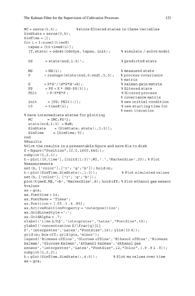
MC = zeros(0,5);
%store filtered states in these variables
SimState = zeros(0,5);
SimTime = [];
for i = 1:numel(timeE)
tspan = [t0 timeE(i)];
[T,state] = ode45(OdeSys, tspan, init);
% simulate / solve model
PS
= state(end,1:5)';
% predicted state
MS
= ME(i);
% measured state
P
= reshape(state(end,6:end),5,5);
% process covariance
% matrix
K
= P*H'/(H*P*H'+R);
% kalman gain matrix
FS
= PS + K * (MS-PS(3));
% filtered state
Pfilt
= P-K*H*P ;
% filtered process
% covariance matrix
init
= [FS; Pfilt(:)];
% new initial condition
t0
= timeE(i);
% new starting time for
% next iteration
% Save intermediate states for plotting
MC
= [MC;FS'];
state(end,1:3) = NaN;
SimState
= [SimState; state(:,1:5)];
SimTime
= [SimTime; T];
end
%Results
%Plot the results in a presentable figure and save file to disk
f = figure("Position",[0,0,1600,640]);
subplot(1,2,1);
h = plot([0,time'],[initX(1:3)';M],'.','MarkerSize',20); % Plot
%measurements
set(h, {'color'},{'r'; 'g';'b'}); hold on;
h = plot(SimTime,SimState(:,1:3));
% Plot simulated values
set(h, {'color'}, {'r'; 'g';'b'});
plot(timeE,ME,'+b','MarkerSize',8); hold off; % Plot ethanol gas sensor
%values
ax = gca;
ax.FontSize = 14;
ax.FontName = 'Times';
ax.Position = [.05 .1 .4 .85];
ax.ActivePositionProperty = 'outerposition';
ax.GridLineStyle =':';
ax.GridAlpha = .7;
xlabel('time $/h$','interpreter','Latex',"FontSize",16);
ylabel('concentration $/\frac{g}{L}
$','interpreter','Latex',"FontSize",16); ylim([0 8]);
grid on; box off; grid(gca,'minor');
legend('Biomass offline','Glucose offline','Ethanol offline','Biomass
Kalman','Glucose Kalman','Ethanol Kalman','Ethanol gas
sensor','interpreter','Latex',"FontSize",12,"Color",[.9 .9 1 .9]);
subplot(1,2,2);
h = plot(SimTime,SimState(:,4:5));
% Plot mu values over time
ax = gca;
The Kalman Filter for the Supervision of Cultivation Processes
121