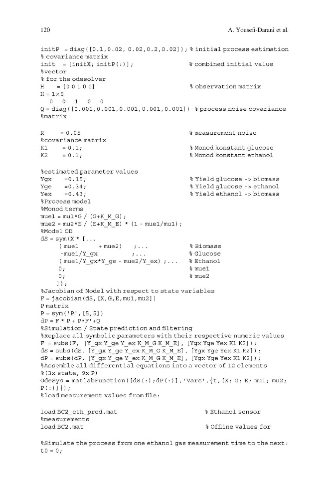
initP = diag([0.1,0.02, 0.02,0.2,0.02]); % initial process estimation
% covariance matrix
init = [initX; initP(:)];
% combined initial value
%vector
% for the odesolver
H
= [0 0 1 0 0]
% observation matrix
H = 1Â5
0 0 1 0 0
Q = diag([0.001,0.001,0.001,0.001,0.001]) % process noise covariance
%matrix
R
= 0.05
% measurement noise
%covariance matrix
K1
= 0.1;
% Monod konstant glucose
K2
= 0.1;
% Monod konstant ethanol
%estimated parameter values
Ygx
=0.15;
% Yield glucose -> biomass
Yge
=0.34;
% Yield glucose -> ethanol
Yex
=0.43;
% Yield ethanol -> biomass
%Process model
%Monod terms
mue1 = mu1*G / (G+K_M_G);
mue2 = mu2*E / (E+K_M_E) * (1 - mue1/mu1);
%Model OD
dS = sym(X * [...
( mue1
+ mue2)
;...
% Biomass
-mue1/Y_gx
;...
% Glucose
( mue1/Y_gx*Y_ge - mue2/Y_ex) ;...
% Ethanol
0;
% mue1
0;
% mue2
]);
%Jacobian of Model with respect to state variables
F = jacobian(dS,[X,G,E,mu1,mu2])
P matrix
P = sym('P',[5,5])
dP = F * P + P*F'+Q
%Simulation / State prediction and filtering
%Replace all symbolic parameters with their respective numeric values
F = subs(F, [Y_gx Y_ge Y_ex K_M_G K_M_E], [Ygx Yge Yex K1 K2]);
dS = subs(dS, [Y_gx Y_ge Y_ex K_M_G K_M_E], [Ygx Yge Yex K1 K2]);
dP = subs(dP, [Y_gx Y_ge Y_ex K_M_G K_M_E], [Ygx Yge Yex K1 K2]);
%Assemble all differential equations into a vector of 12 elements
%(3x state, 9x P)
OdeSys = matlabFunction([dS(:);dP(:)],'Vars',{t,[X; G; E; mu1; mu2;
P(:)]});
%load measurement values from file:
load BC2_eth_pred.mat
% Ethanol sensor
%measurements
load BC2.mat
% Offline values for
%Simulate the process from one ethanol gas measurement time to the next:
t0 = 0;
120
A. Yousefi-Darani et al.