

64
3 Hypothetical Objects in Electromagnetism and Gravity
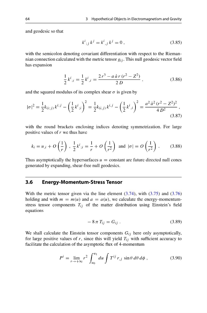
and geodesic so that
k
i ;j k
j
= k
i
,j k
j
= 0 ,
(3.85)
with the semicolon denoting covariant differentiation with respect to the Riemannian connection calculated with the metric tensor g ij . This null geodesic vector field
has expansion
1
2
k
i ;i =
1
2
k
i
,i =
2 r 3 − a ˙
a r (r 2 − Z 2 )
2 D
,
(3.86)
and the squared modulus of its complex shear σ is given by
|σ |
2
=
1
2
k (i;j) k
i;j
−
1
2
k
i ;i
2
=
1
2
k (i,j ) k
i,j
−
1
2
k
i
,i
2
=
a 2 ˙
a 2 (r 2 − Z 2 ) 2
4 D 2
,
(3.87)
with the round brackets enclosing indices denoting symmetrization. For large
positive values of r we thus have
k i = u ,i + O
1
r
,
1
2
k
i ;i =
1
r
+ O
1
r 2
and |σ | = O
1
r 2
.
(3.88)
Thus asymptotically the hypersurfaces u = constant are future directed null cones
generated by expanding, shear-free null geodesics.
3.6
Energy-Momentum-Stress Tensor
With the metric tensor given via the line element (3.74), with (3.75) and (3.76)
holding and with m = m(u) and a = a(u), we calculate the energy-momentumstress tensor components T ij of the matter distribution using Einstein’s field
equations
− 8 π T ij = G ij .
(3.89)
We shall calculate the Einstein tensor components G ij here only asymptotically,
for large positive values of r, since this will yield T ij with sufficient accuracy to
facilitate the calculation of the asymptotic flux of 4-momentum
P
i
= lim
r→+∞
r
2
u 1
u 0
du
T
ij r ,j sin θ dθ dφ ,
(3.90)
3 Hypothetical Objects in Electromagnetism and Gravity
and geodesic so that
k
i ;j k
j
= k
i
,j k
j
= 0 ,
(3.85)
with the semicolon denoting covariant differentiation with respect to the Riemannian connection calculated with the metric tensor g ij . This null geodesic vector field
has expansion
1
2
k
i ;i =
1
2
k
i
,i =
2 r 3 − a ˙
a r (r 2 − Z 2 )
2 D
,
(3.86)
and the squared modulus of its complex shear σ is given by
|σ |
2
=
1
2
k (i;j) k
i;j
−
1
2
k
i ;i
2
=
1
2
k (i,j ) k
i,j
−
1
2
k
i
,i
2
=
a 2 ˙
a 2 (r 2 − Z 2 ) 2
4 D 2
,
(3.87)
with the round brackets enclosing indices denoting symmetrization. For large
positive values of r we thus have
k i = u ,i + O
1
r
,
1
2
k
i ;i =
1
r
+ O
1
r 2
and |σ | = O
1
r 2
.
(3.88)
Thus asymptotically the hypersurfaces u = constant are future directed null cones
generated by expanding, shear-free null geodesics.
3.6
Energy-Momentum-Stress Tensor
With the metric tensor given via the line element (3.74), with (3.75) and (3.76)
holding and with m = m(u) and a = a(u), we calculate the energy-momentumstress tensor components T ij of the matter distribution using Einstein’s field
equations
− 8 π T ij = G ij .
(3.89)
We shall calculate the Einstein tensor components G ij here only asymptotically,
for large positive values of r, since this will yield T ij with sufficient accuracy to
facilitate the calculation of the asymptotic flux of 4-momentum
P
i
= lim
r→+∞
r
2
u 1
u 0
du
T
ij r ,j sin θ dθ dφ ,
(3.90)