

62
3 Hypothetical Objects in Electromagnetism and Gravity
For comparison purposes later we note that the Einstein tensor components G ij =
R ij −
1
2 g ij R, with R = g ij R ij the Ricci scalar, read
G ij =
2 ˙
m
r 2 k i k j = −8 π T ij ,
(3.73)
where T ij are the components of the energy-momentum-stress tensor of a matter
distribution. Eq.(3.73) represents Einstein’s field equations in the current context.
The matter distribution here consists of particles travelling with the speed of light
radially away from the isolated spherical source.
Following the pattern established here of starting with the Kerr–Schild form
(3.65) of the Schwarzschild line element, identifying a variable u using (3.70), and
then using it to generalise the Schwarzschild line element, we wish to apply this to
the axisymmetric Kerr line element [8]. There is a literature on the generalisation
of the Vaidya space-time to axial symmetry which has been summarised in [9] as
follows: “In the axisymmetric case, the complete solution was first found by Herlt
[10], using a formalism developed by Vaidya [11, 12]”. The Herlt solution includes
the so-called “radiating Kerr metric” constructed by Vaidya and Patel [13]. It is
importantly emphasised in [9] that none of the non-vacuum solutions of this type
can be interpreted as having a pure radiation Maxwell field as source. The Vaidya
solution has continued to stimulate research (see for example [14–18]).
3.5
Axial Symmetry
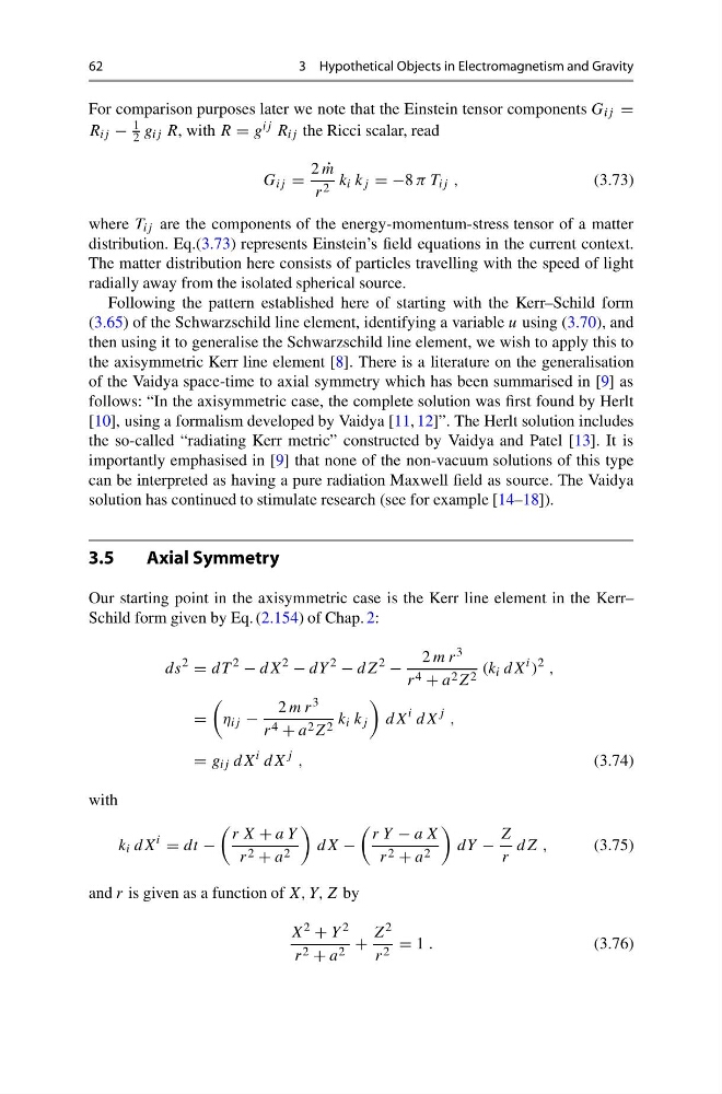
Our starting point in the axisymmetric case is the Kerr line element in the Kerr–
Schild form given by Eq. (2.154) of Chap. 2:
ds
2
= dT
2
− dX
2
− dY
2
− dZ
2
−
2 m r 3
r 4 + a 2 Z 2 (k i dX
i )
2 ,
=
η ij −
2 m r 3
r 4 + a 2 Z 2 k i k j
dX
i dX
j ,
= g ij dX
i dX
j ,
(3.74)
with
k i dX
i
= dt −
r X + a Y
r 2 + a 2
dX −
r Y − a X
r 2 + a 2
dY −
Z
r
dZ ,
(3.75)
and r is given as a function of X, Y, Z by
X 2 + Y 2
r 2 + a 2 +
Z 2
r 2 = 1 .
(3.76)
3 Hypothetical Objects in Electromagnetism and Gravity
For comparison purposes later we note that the Einstein tensor components G ij =
R ij −
1
2 g ij R, with R = g ij R ij the Ricci scalar, read
G ij =
2 ˙
m
r 2 k i k j = −8 π T ij ,
(3.73)
where T ij are the components of the energy-momentum-stress tensor of a matter
distribution. Eq.(3.73) represents Einstein’s field equations in the current context.
The matter distribution here consists of particles travelling with the speed of light
radially away from the isolated spherical source.
Following the pattern established here of starting with the Kerr–Schild form
(3.65) of the Schwarzschild line element, identifying a variable u using (3.70), and
then using it to generalise the Schwarzschild line element, we wish to apply this to
the axisymmetric Kerr line element [8]. There is a literature on the generalisation
of the Vaidya space-time to axial symmetry which has been summarised in [9] as
follows: “In the axisymmetric case, the complete solution was first found by Herlt
[10], using a formalism developed by Vaidya [11, 12]”. The Herlt solution includes
the so-called “radiating Kerr metric” constructed by Vaidya and Patel [13]. It is
importantly emphasised in [9] that none of the non-vacuum solutions of this type
can be interpreted as having a pure radiation Maxwell field as source. The Vaidya
solution has continued to stimulate research (see for example [14–18]).
3.5
Axial Symmetry
Our starting point in the axisymmetric case is the Kerr line element in the Kerr–
Schild form given by Eq. (2.154) of Chap. 2:
ds
2
= dT
2
− dX
2
− dY
2
− dZ
2
−
2 m r 3
r 4 + a 2 Z 2 (k i dX
i )
2 ,
=
η ij −
2 m r 3
r 4 + a 2 Z 2 k i k j
dX
i dX
j ,
= g ij dX
i dX
j ,
(3.74)
with
k i dX
i
= dt −
r X + a Y
r 2 + a 2
dX −
r Y − a X
r 2 + a 2
dY −
Z
r
dZ ,
(3.75)
and r is given as a function of X, Y, Z by
X 2 + Y 2
r 2 + a 2 +
Z 2
r 2 = 1 .
(3.76)