

30
2 Bivector Formalism
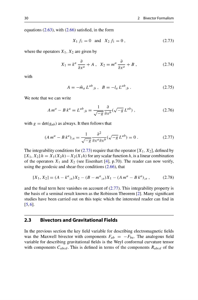
equations (2.63), with (2.66) satisfied, in the form
X 1 f 1 = 0 and X 2 f 1 = 0 ,
(2.73)
where the operators X 1 , X 2 are given by
X 1 = k
a ∂
∂x a + A , X 2 = m
a ∂
∂x a + B ,
(2.74)
with
A = − ¯
m a L
ab ;b , B = −l a L
ab ;b .
(2.75)
We note that we can write
A m
a
− B k
a
= L
ab ;b =
1
√
−g
∂
∂x b (
√ −g L
ab ) ,
(2.76)
with g = det(g ab ) as always. It then follows that
(A m
a
− B k
a ) ;a =
1
√ −g
∂ 2
∂x a ∂x b (
√ −g L
ab ) = 0 .
(2.77)
The integrability conditions for (2.73) require that the operator [X 1 , X 2 ], defined by
[X 1 , X 2 ] h = X 1 (X 2 h)−X 2 (X 1 h) for any scalar function h, is a linear combination
of the operators X 1 and X 2 (see Eisenhart [4], p.70). The reader can now verify,
using the geodesic and shear-free conditions (2.66), that
[X 1 , X 2 ] = (A − k
a ;a )X 2 − (B − m
a ;a )X 1 − (A m
a
− B k
a ) ;a ,
(2.78)
and the final term here vanishes on account of (2.77). This integrability property is
the basis of a seminal result known as the Robinson Theorem [2]. Many significant
studies have been carried out on this topic which the interested reader can find in
[5, 6].
2.3
Bivectors and Gravitational Fields
In the previous section the key field variable for describing electromagnetic fields
was the Maxwell bivector with components F ab = −F ba . The analogous field
variable for describing gravitational fields is the Weyl conformal curvature tensor
with components C abcd . This is defined in terms of the components R abcd of the
2 Bivector Formalism
equations (2.63), with (2.66) satisfied, in the form
X 1 f 1 = 0 and X 2 f 1 = 0 ,
(2.73)
where the operators X 1 , X 2 are given by
X 1 = k
a ∂
∂x a + A , X 2 = m
a ∂
∂x a + B ,
(2.74)
with
A = − ¯
m a L
ab ;b , B = −l a L
ab ;b .
(2.75)
We note that we can write
A m
a
− B k
a
= L
ab ;b =
1
√
−g
∂
∂x b (
√ −g L
ab ) ,
(2.76)
with g = det(g ab ) as always. It then follows that
(A m
a
− B k
a ) ;a =
1
√ −g
∂ 2
∂x a ∂x b (
√ −g L
ab ) = 0 .
(2.77)
The integrability conditions for (2.73) require that the operator [X 1 , X 2 ], defined by
[X 1 , X 2 ] h = X 1 (X 2 h)−X 2 (X 1 h) for any scalar function h, is a linear combination
of the operators X 1 and X 2 (see Eisenhart [4], p.70). The reader can now verify,
using the geodesic and shear-free conditions (2.66), that
[X 1 , X 2 ] = (A − k
a ;a )X 2 − (B − m
a ;a )X 1 − (A m
a
− B k
a ) ;a ,
(2.78)
and the final term here vanishes on account of (2.77). This integrability property is
the basis of a seminal result known as the Robinson Theorem [2]. Many significant
studies have been carried out on this topic which the interested reader can find in
[5, 6].
2.3
Bivectors and Gravitational Fields
In the previous section the key field variable for describing electromagnetic fields
was the Maxwell bivector with components F ab = −F ba . The analogous field
variable for describing gravitational fields is the Weyl conformal curvature tensor
with components C abcd . This is defined in terms of the components R abcd of the