

8
1 C o n g r u e n c e s o f W o r l d L i n e s
1.2
Null Geodesic Congruences
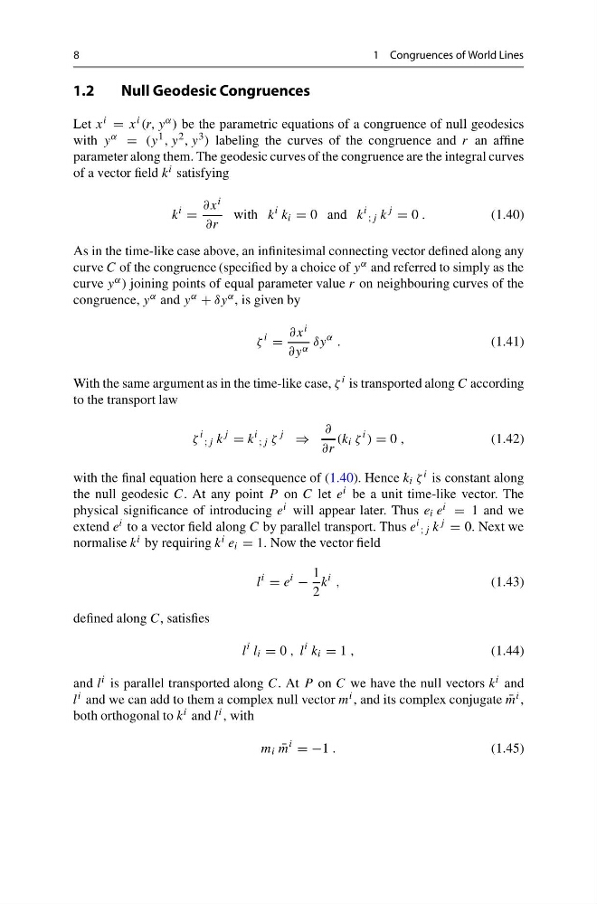
Let x i = x i (r, y α ) be the parametric equations of a congruence of null geodesics
with y α = (y 1 , y 2 , y 3 ) labeling the curves of the congruence and r an affine
parameter along them. The geodesic curves of the congruence are the integral curves
of a vector field k i satisfying
k
i
=
∂x i
∂r
with k
i k i = 0 and k
i ;j k
j
= 0 .
(1.40)
As in the time-like case above, an infinitesimal connecting vector defined along any
curve C of the congruence (specified by a choice of y α and referred to simply as the
curve y α ) joining points of equal parameter value r on neighbouring curves of the
congruence, y α and y α + δy α , is given by
ζ
i
=
∂x i
∂y α δy
α .
(1.41)
With the same argument as in the time-like case, ζ i is transported along C according
to the transport law
ζ
i ;j k
j
= k
i ;j ζ
j
⇒
∂
∂r
(k i ζ
i ) = 0 ,
(1.42)
with the final equation here a consequence of (1.40). Hence k i ζ i is constant along
the null geodesic C. At any point P on C let e i be a unit time-like vector. The
physical significance of introducing e i will appear later. Thus e i e i = 1 and we
extend e i to a vector field along C by parallel transport. Thus e i ;j k j = 0. Next we
normalise k i by requiring k i e i = 1. Now the vector field
l
i
= e
i
−
1
2
k
i ,
(1.43)
defined along C, satisfies
l
i l i = 0 , l
i k i = 1 ,
(1.44)
and l i is parallel transported along C. At P on C we have the null vectors k i and
l i and we can add to them a complex null vector m i , and its complex conjugate ¯
m i ,
both orthogonal to k i and l i , with
m i ¯
m
i
= −1 .
(1.45)
1 C o n g r u e n c e s o f W o r l d L i n e s
1.2
Null Geodesic Congruences
Let x i = x i (r, y α ) be the parametric equations of a congruence of null geodesics
with y α = (y 1 , y 2 , y 3 ) labeling the curves of the congruence and r an affine
parameter along them. The geodesic curves of the congruence are the integral curves
of a vector field k i satisfying
k
i
=
∂x i
∂r
with k
i k i = 0 and k
i ;j k
j
= 0 .
(1.40)
As in the time-like case above, an infinitesimal connecting vector defined along any
curve C of the congruence (specified by a choice of y α and referred to simply as the
curve y α ) joining points of equal parameter value r on neighbouring curves of the
congruence, y α and y α + δy α , is given by
ζ
i
=
∂x i
∂y α δy
α .
(1.41)
With the same argument as in the time-like case, ζ i is transported along C according
to the transport law
ζ
i ;j k
j
= k
i ;j ζ
j
⇒
∂
∂r
(k i ζ
i ) = 0 ,
(1.42)
with the final equation here a consequence of (1.40). Hence k i ζ i is constant along
the null geodesic C. At any point P on C let e i be a unit time-like vector. The
physical significance of introducing e i will appear later. Thus e i e i = 1 and we
extend e i to a vector field along C by parallel transport. Thus e i ;j k j = 0. Next we
normalise k i by requiring k i e i = 1. Now the vector field
l
i
= e
i
−
1
2
k
i ,
(1.43)
defined along C, satisfies
l
i l i = 0 , l
i k i = 1 ,
(1.44)
and l i is parallel transported along C. At P on C we have the null vectors k i and
l i and we can add to them a complex null vector m i , and its complex conjugate ¯
m i ,
both orthogonal to k i and l i , with
m i ¯
m
i
= −1 .
(1.45)