

7.2 Background Space-Time/External Fields
159
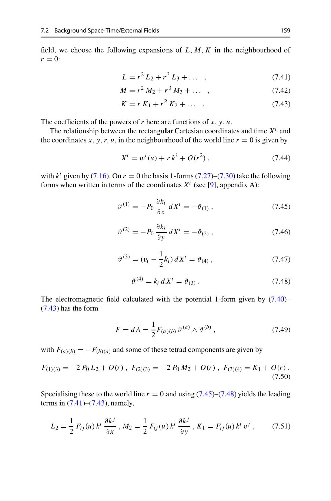
field, we choose the following expansions of L, M, K in the neighbourhood of
r = 0:
L = r
2 L 2 + r
3 L 3 + . . . ,
(7.41)
M = r
2 M 2 + r
3 M 3 + . . . ,
(7.42)
K = r K 1 + r
2 K 2 + . . . .
(7.43)
The coefficients of the powers of r here are functions of x, y, u.
The relationship between the rectangular Cartesian coordinates and time X i and
the coordinates x, y, r, u, in the neighbourhood of the world line r = 0 is given by
X
i
= w
i (u) + r k
i
+ O(r
2 ) ,
(7.44)
with k i given by (7.16). On r = 0 the basis 1-forms (7.27)–(7.30) take the following
forms when written in terms of the coordinates X i (see [9], appendix A):
ϑ
(1)
= −P 0
∂k i
∂x
dX
i
= −ϑ (1) ,
(7.45)
ϑ
(2)
= −P 0
∂k i
∂y
dX
i
= −ϑ (2) ,
(7.46)
ϑ
(3)
= (v i −
1
2
k i ) dX
i
= ϑ (4) ,
(7.47)
ϑ
(4)
= k i dX
i
= ϑ (3) .
(7.48)
The electromagnetic field calculated with the potential 1-form given by (7.40)–
(7.43) has the form
F = dA =
1
2
F (a)(b) ϑ
(a)
∧ ϑ
(b) ,
(7.49)
with F (a)(b) = −F (b)(a) and some of these tetrad components are given by
F (1)(3) = −2 P 0 L 2 + O(r) , F (2)(3) = −2 P 0 M 2 + O(r) , F (3)(4) = K 1 + O(r) .
(7.50)
Specialising these to the world line r = 0 and using (7.45)–(7.48) yields the leading
terms in (7.41)–(7.43), namely,
L 2 =
1
2
F ij (u) k
i ∂k j
∂x
, M 2 =
1
2
F ij (u) k
i ∂k j
∂y
, K 1 = F ij (u) k
i v
j ,
(7.51)
159
field, we choose the following expansions of L, M, K in the neighbourhood of
r = 0:
L = r
2 L 2 + r
3 L 3 + . . . ,
(7.41)
M = r
2 M 2 + r
3 M 3 + . . . ,
(7.42)
K = r K 1 + r
2 K 2 + . . . .
(7.43)
The coefficients of the powers of r here are functions of x, y, u.
The relationship between the rectangular Cartesian coordinates and time X i and
the coordinates x, y, r, u, in the neighbourhood of the world line r = 0 is given by
X
i
= w
i (u) + r k
i
+ O(r
2 ) ,
(7.44)
with k i given by (7.16). On r = 0 the basis 1-forms (7.27)–(7.30) take the following
forms when written in terms of the coordinates X i (see [9], appendix A):
ϑ
(1)
= −P 0
∂k i
∂x
dX
i
= −ϑ (1) ,
(7.45)
ϑ
(2)
= −P 0
∂k i
∂y
dX
i
= −ϑ (2) ,
(7.46)
ϑ
(3)
= (v i −
1
2
k i ) dX
i
= ϑ (4) ,
(7.47)
ϑ
(4)
= k i dX
i
= ϑ (3) .
(7.48)
The electromagnetic field calculated with the potential 1-form given by (7.40)–
(7.43) has the form
F = dA =
1
2
F (a)(b) ϑ
(a)
∧ ϑ
(b) ,
(7.49)
with F (a)(b) = −F (b)(a) and some of these tetrad components are given by
F (1)(3) = −2 P 0 L 2 + O(r) , F (2)(3) = −2 P 0 M 2 + O(r) , F (3)(4) = K 1 + O(r) .
(7.50)
Specialising these to the world line r = 0 and using (7.45)–(7.48) yields the leading
terms in (7.41)–(7.43), namely,
L 2 =
1
2
F ij (u) k
i ∂k j
∂x
, M 2 =
1
2
F ij (u) k
i ∂k j
∂y
, K 1 = F ij (u) k
i v
j ,
(7.51)