

5.4 Gravitational Clock Compass
121
Plane Gravitational Waves
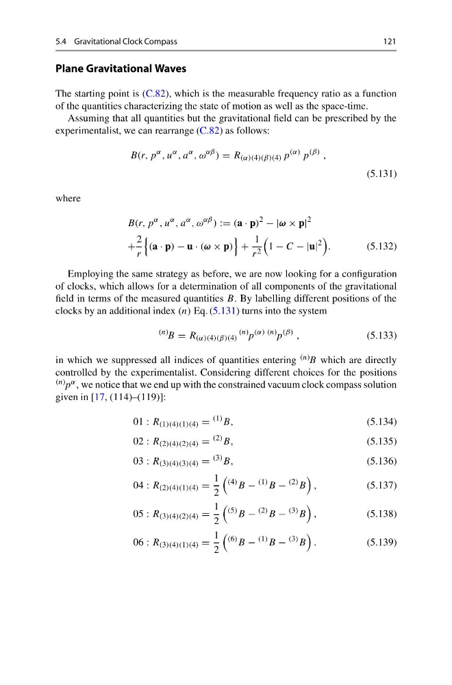
The starting point is (C.82), which is the measurable frequency ratio as a function
of the quantities characterizing the state of motion as well as the space-time.
Assuming that all quantities but the gravitational field can be prescribed by the
experimentalist, we can rearrange (C.82) as follows:
B(r, p
α , u
α , a
α , ω
αβ ) = R (α)(4)(β)(4) p
(α) p
(β) ,
(5.131)
where
B(r, p
α , u
α , a
α , ω
αβ ) := (a · p)
2
− |ω × p|
2
+
2
r
(a · p) − u · (ω × p)
+
1
r 2
1 − C − |u|
2
.
(5.132)
Employing the same strategy as before, we are now looking for a configuration
of clocks, which allows for a determination of all components of the gravitational
field in terms of the measured quantities B. By labelling different positions of the
clocks by an additional index (n) Eq. (5.131) turns into the system
(n)
B = R (α)(4)(β)(4)
(n)
p
(α) (n)
p
(β) ,
(5.133)
in which we suppressed all indices of quantities entering (n) B which are directly
controlled by the experimentalist. Considering different choices for the positions
(n) p α , we notice that we end up with the constrained vacuum clock compass solution
given in [17, (114)–(119)]:
01 : R (1)(4)(1)(4) =
(1) B,
(5.134)
02 : R (2)(4)(2)(4) =
(2) B,
(5.135)
03 : R (3)(4)(3)(4) =
(3) B,
(5.136)
04 : R (2)(4)(1)(4) =
1
2
(4) B −
(1) B −
(2) B
,
(5.137)
05 : R (3)(4)(2)(4) =
1
2
(5) B −
(2) B −
(3) B
,
(5.138)
06 : R (3)(4)(1)(4) =
1
2
(6) B −
(1) B −
(3) B
.
(5.139)
121
Plane Gravitational Waves
The starting point is (C.82), which is the measurable frequency ratio as a function
of the quantities characterizing the state of motion as well as the space-time.
Assuming that all quantities but the gravitational field can be prescribed by the
experimentalist, we can rearrange (C.82) as follows:
B(r, p
α , u
α , a
α , ω
αβ ) = R (α)(4)(β)(4) p
(α) p
(β) ,
(5.131)
where
B(r, p
α , u
α , a
α , ω
αβ ) := (a · p)
2
− |ω × p|
2
+
2
r
(a · p) − u · (ω × p)
+
1
r 2
1 − C − |u|
2
.
(5.132)
Employing the same strategy as before, we are now looking for a configuration
of clocks, which allows for a determination of all components of the gravitational
field in terms of the measured quantities B. By labelling different positions of the
clocks by an additional index (n) Eq. (5.131) turns into the system
(n)
B = R (α)(4)(β)(4)
(n)
p
(α) (n)
p
(β) ,
(5.133)
in which we suppressed all indices of quantities entering (n) B which are directly
controlled by the experimentalist. Considering different choices for the positions
(n) p α , we notice that we end up with the constrained vacuum clock compass solution
given in [17, (114)–(119)]:
01 : R (1)(4)(1)(4) =
(1) B,
(5.134)
02 : R (2)(4)(2)(4) =
(2) B,
(5.135)
03 : R (3)(4)(3)(4) =
(3) B,
(5.136)
04 : R (2)(4)(1)(4) =
1
2
(4) B −
(1) B −
(2) B
,
(5.137)
05 : R (3)(4)(2)(4) =
1
2
(5) B −
(2) B −
(3) B
,
(5.138)
06 : R (3)(4)(1)(4) =
1
2
(6) B −
(1) B −
(3) B
.
(5.139)