

5.2 Gravitational Compass
101
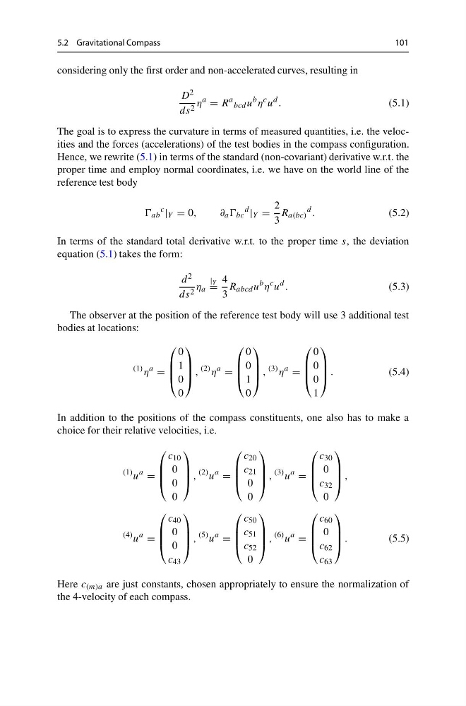
considering only the first order and non-accelerated curves, resulting in
D 2
ds 2 η
a
= R
a
bcd u
b η
c u
d .
(5.1)
The goal is to express the curvature in terms of measured quantities, i.e. the velocities and the forces (accelerations) of the test bodies in the compass configuration.
Hence, we rewrite (5.1) in terms of the standard (non-covariant) derivative w.r.t. the
proper time and employ normal coordinates, i.e. we have on the world line of the
reference test body
ab
c
| Y = 0,
∂ a bc
d
| Y =
2
3
R a(bc)
d .
(5.2)
In terms of the standard total derivative w.r.t. to the proper time s, the deviation
equation (5.1) takes the form:
d 2
ds 2 η a
| Y
=
4
3
R abcd u
b η
c u
d .
(5.3)
The observer at the position of the reference test body will use 3 additional test
bodies at locations:
(1) η
a
=
⎛
⎜
⎜
⎝
0
1
0
0
⎞
⎟
⎟
⎠ ,
(2) η
a
=
⎛
⎜
⎜
⎝
0
0
1
0
⎞
⎟
⎟
⎠ ,
(3) η
a
=
⎛
⎜
⎜
⎝
0
0
0
1
⎞
⎟
⎟
⎠ .
(5.4)
In addition to the positions of the compass constituents, one also has to make a
choice for their relative velocities, i.e.
(1) u
a
=
⎛
⎜
⎜
⎝
c 10
0
0
0
⎞
⎟
⎟
⎠ ,
(2) u
a
=
⎛
⎜
⎜
⎝
c 20
c 21
0
0
⎞
⎟
⎟
⎠ ,
(3) u
a
=
⎛
⎜
⎜
⎝
c 30
0
c 32
0
⎞
⎟
⎟
⎠ ,
(4) u
a
=
⎛
⎜
⎜
⎝
c 40
0
0
c 43
⎞
⎟
⎟
⎠ ,
(5) u
a
=
⎛
⎜
⎜
⎝
c 50
c 51
c 52
0
⎞
⎟
⎟
⎠ ,
(6) u
a
=
⎛
⎜
⎜
⎝
c 60
0
c 62
c 63
⎞
⎟
⎟
⎠ .
(5.5)
Here c (m)a are just constants, chosen appropriately to ensure the normalization of
the 4-velocity of each compass.
101
considering only the first order and non-accelerated curves, resulting in
D 2
ds 2 η
a
= R
a
bcd u
b η
c u
d .
(5.1)
The goal is to express the curvature in terms of measured quantities, i.e. the velocities and the forces (accelerations) of the test bodies in the compass configuration.
Hence, we rewrite (5.1) in terms of the standard (non-covariant) derivative w.r.t. the
proper time and employ normal coordinates, i.e. we have on the world line of the
reference test body
ab
c
| Y = 0,
∂ a bc
d
| Y =
2
3
R a(bc)
d .
(5.2)
In terms of the standard total derivative w.r.t. to the proper time s, the deviation
equation (5.1) takes the form:
d 2
ds 2 η a
| Y
=
4
3
R abcd u
b η
c u
d .
(5.3)
The observer at the position of the reference test body will use 3 additional test
bodies at locations:
(1) η
a
=
⎛
⎜
⎜
⎝
0
1
0
0
⎞
⎟
⎟
⎠ ,
(2) η
a
=
⎛
⎜
⎜
⎝
0
0
1
0
⎞
⎟
⎟
⎠ ,
(3) η
a
=
⎛
⎜
⎜
⎝
0
0
0
1
⎞
⎟
⎟
⎠ .
(5.4)
In addition to the positions of the compass constituents, one also has to make a
choice for their relative velocities, i.e.
(1) u
a
=
⎛
⎜
⎜
⎝
c 10
0
0
0
⎞
⎟
⎟
⎠ ,
(2) u
a
=
⎛
⎜
⎜
⎝
c 20
c 21
0
0
⎞
⎟
⎟
⎠ ,
(3) u
a
=
⎛
⎜
⎜
⎝
c 30
0
c 32
0
⎞
⎟
⎟
⎠ ,
(4) u
a
=
⎛
⎜
⎜
⎝
c 40
0
0
c 43
⎞
⎟
⎟
⎠ ,
(5) u
a
=
⎛
⎜
⎜
⎝
c 50
c 51
c 52
0
⎞
⎟
⎟
⎠ ,
(6) u
a
=
⎛
⎜
⎜
⎝
c 60
0
c 62
c 63
⎞
⎟
⎟
⎠ .
(5.5)
Here c (m)a are just constants, chosen appropriately to ensure the normalization of
the 4-velocity of each compass.