

6.4 Multi-level Wavelet CNN for Image Restoration in Pre-Processing Sub-System
221
of ADMM and HQS [28] to solve the fidelity term and the regularization term. All
of the above methods show that the decoupling of the fidelity term and the regularization term enables various existing models to solve different image restoration
tasks.
6.4.2 Half Quadratic Splitting (HQS)
Generally speaking, the fidelity term and regularization term are decoupled by the
variable splitting technique to plug the denoiser prior to Eq. (2)’s optimization
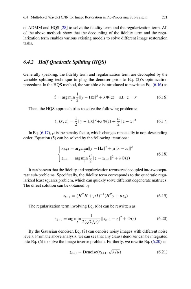
procedure. In the HQS method, the variable z is introduced to rewritten Eq. (6.16) as
ˆ
x = arg min
x
1
2
y − Hx
2
+ λλ(z) s.t. z = x
(6.16)
Then, the HQS approach tries to solve the following problems:
μ (x, z) =
1
2
y − Hx
2
+λλ(z) +
μ
2
z − x
2
(6.17)
In Eq. (6.17), μ is the penalty factor, which changes repeatedly in non-descending
order. Equation (5) can be solved by the following iterations:
⎧
⎨
⎩
x k+1 = arg min
x
y − Hx
2
+ μx − z k
2
z k+1 = arg min
z
μ
2
z − x k+1
2
+ λλ(z)
(6.18)
It can be seen that the fidelity and regularization terms are decoupled into two separate sub-problems. Specifically, the fidelity term corresponds to the quadratic regularized least squares problem, which can quickly solve different degenerate matrices.
The direct solution can be obtained by
x k+1 = (H
T H + μI )
−1
(H
T y + μz k )
(6.19)
The regularization term involving Eq. (6b) can be rewritten as
z k+1 = arg min
x
1
2(
√ λ/μ) 2 x k+1 − z
2
+ (z)
(6.20)
By the Gaussian denoiser, Eq. (8) can denoise noisy images with different noise
levels. From the above analysis, we can see that any Gauss denoiser can be integrated
into Eq. (6) to solve the image inverse problem. Furtherly, we rewrite Eq. (6.20) as
z k+1 = Denoise(x k+1 ,
λ/μ)
(6.21)
221
of ADMM and HQS [28] to solve the fidelity term and the regularization term. All
of the above methods show that the decoupling of the fidelity term and the regularization term enables various existing models to solve different image restoration
tasks.
6.4.2 Half Quadratic Splitting (HQS)
Generally speaking, the fidelity term and regularization term are decoupled by the
variable splitting technique to plug the denoiser prior to Eq. (2)’s optimization
procedure. In the HQS method, the variable z is introduced to rewritten Eq. (6.16) as
ˆ
x = arg min
x
1
2
y − Hx
2
+ λλ(z) s.t. z = x
(6.16)
Then, the HQS approach tries to solve the following problems:
μ (x, z) =
1
2
y − Hx
2
+λλ(z) +
μ
2
z − x
2
(6.17)
In Eq. (6.17), μ is the penalty factor, which changes repeatedly in non-descending
order. Equation (5) can be solved by the following iterations:
⎧
⎨
⎩
x k+1 = arg min
x
y − Hx
2
+ μx − z k
2
z k+1 = arg min
z
μ
2
z − x k+1
2
+ λλ(z)
(6.18)
It can be seen that the fidelity and regularization terms are decoupled into two separate sub-problems. Specifically, the fidelity term corresponds to the quadratic regularized least squares problem, which can quickly solve different degenerate matrices.
The direct solution can be obtained by
x k+1 = (H
T H + μI )
−1
(H
T y + μz k )
(6.19)
The regularization term involving Eq. (6b) can be rewritten as
z k+1 = arg min
x
1
2(
√ λ/μ) 2 x k+1 − z
2
+ (z)
(6.20)
By the Gaussian denoiser, Eq. (8) can denoise noisy images with different noise
levels. From the above analysis, we can see that any Gauss denoiser can be integrated
into Eq. (6) to solve the image inverse problem. Furtherly, we rewrite Eq. (6.20) as
z k+1 = Denoise(x k+1 ,
λ/μ)
(6.21)