

180
5 Optimization Algorithm and RFID System Physical Anti-Collision
max
⎡
⎣ −
1
2
k
i, j=1
(α i − α
∗
i )(α j − α
∗
j )(x i · x j )
−ε
k
i=1
(α i + α
∗
i ) +
k
i=1
y i (α
∗
i − α i )
s.t.
⎧
⎨
⎩
k
i, j=1
(α i − α
∗
i ) = 0
α i , α
∗
i ∈ [0, C]
(5.37)
where α i and α
∗
i are Lagrange factors.
Regression function could be changed into high dimension via the kernel function
K (x i · x j ):
f (x) = ω · x + b =
k
i, j=1
(α
∗
i − α i )K (x i · x j ) + b
∗
(5.38)
(2) Predicted reading distance of tags based on SVM
In this paper, we analyzed the position of tags and the corresponding reading
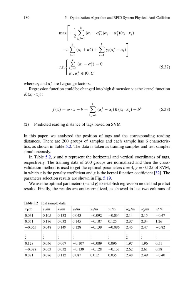
distances. There are 200 groups of samples and each sample has 6 characteristics, as shown in Table 5.2. The data is taken as training samples and test samples
simultaneously.
In Table 5.2, x and y represent the horizontal and vertical coordinates of tags,
respectively. The training data of 200 groups are normalized and then the crossvalidation method is used to get the optimal parameters c = 4, g = 0.125 of SVM,
in which c is the penalty coefficient and g is the kernel function coefficient [32]. The
parameter selection results are shown in Fig. 5.19.
We use the optimal parameters (c and g) to establish regression model and predict
results. Finally, the results are anti-normalized, as showed in last two columns of
Table 5.2 Test sample data
x 1 /m
y 1 /m
x 2 /m
y 2 /m
x 3 /m
y 3 /m
R m /m
R p /m
η/ %
0.031
0.105
0.132
0.043
−0.092
−0.034
2.14
2.15
−0.47
0.051
0.176
0.032
0.145
−0.107
0.125
2.37
2.34
1.26
−0.065
0.048
0.149
0.128
−0.139
−0.086
2.45
2.47
−0.82
. . .
. . .
. . .
. . .
. . .
. . .
. . .
. . .
. . .
. . .
0.128
0.036
0.067
−0.107
−0.089
0.096
1.97
1.96
0.51
−0.078
0.063
0.032
−0.139
−0.128
−0.137
2.62
2.61
0.38
0.021
0.076
0.112
0.087
0.012
0.035
2.48
2.49
−0.40
5 Optimization Algorithm and RFID System Physical Anti-Collision
max
⎡
⎣ −
1
2
k
i, j=1
(α i − α
∗
i )(α j − α
∗
j )(x i · x j )
−ε
k
i=1
(α i + α
∗
i ) +
k
i=1
y i (α
∗
i − α i )
s.t.
⎧
⎨
⎩
k
i, j=1
(α i − α
∗
i ) = 0
α i , α
∗
i ∈ [0, C]
(5.37)
where α i and α
∗
i are Lagrange factors.
Regression function could be changed into high dimension via the kernel function
K (x i · x j ):
f (x) = ω · x + b =
k
i, j=1
(α
∗
i − α i )K (x i · x j ) + b
∗
(5.38)
(2) Predicted reading distance of tags based on SVM
In this paper, we analyzed the position of tags and the corresponding reading
distances. There are 200 groups of samples and each sample has 6 characteristics, as shown in Table 5.2. The data is taken as training samples and test samples
simultaneously.
In Table 5.2, x and y represent the horizontal and vertical coordinates of tags,
respectively. The training data of 200 groups are normalized and then the crossvalidation method is used to get the optimal parameters c = 4, g = 0.125 of SVM,
in which c is the penalty coefficient and g is the kernel function coefficient [32]. The
parameter selection results are shown in Fig. 5.19.
We use the optimal parameters (c and g) to establish regression model and predict
results. Finally, the results are anti-normalized, as showed in last two columns of
Table 5.2 Test sample data
x 1 /m
y 1 /m
x 2 /m
y 2 /m
x 3 /m
y 3 /m
R m /m
R p /m
η/ %
0.031
0.105
0.132
0.043
−0.092
−0.034
2.14
2.15
−0.47
0.051
0.176
0.032
0.145
−0.107
0.125
2.37
2.34
1.26
−0.065
0.048
0.149
0.128
−0.139
−0.086
2.45
2.47
−0.82
. . .
. . .
. . .
. . .
. . .
. . .
. . .
. . .
. . .
. . .
0.128
0.036
0.067
−0.107
−0.089
0.096
1.97
1.96
0.51
−0.078
0.063
0.032
−0.139
−0.128
−0.137
2.62
2.61
0.38
0.021
0.076
0.112
0.087
0.012
0.035
2.48
2.49
−0.40