

166
5 Optimization Algorithm and RFID System Physical Anti-Collision
Table 5.1 The training data and results of PSO neural network
x 1 /m
y 1 /m
z 1 /m
…
x 7 /m
y 7 /m
z 7 /m
d r /m
d p /m
E/%
0.815
0.278
0.216
…
0.957
0.592
0.235
1.23
1.22
0.81
0.906
0.547
0.189
…
0.485
0.759
0.191
1.65
1.67
1.21
0.127
0.957
0.117
…
0.800
0.655
0.170
0.96
0.95
1.04
. . .
. . .
. . .
. . .
. . .
. . .
. . .
. . .
. . .
0.913
0.962
0.165
…
0.142
0.135
0.065
1.11
1.11
0
0.632
0.157
0.203
…
0.426
0.849
0.158
1.36
1.37
0.74
0.097
0.970
0.079
…
0.915
0.633
0.149
1.68
1.69
0.6
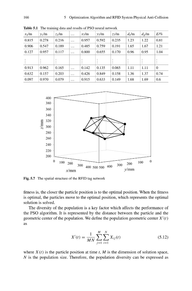
Fig. 5.7 The spatial structure of the RFID tag network
fitness is, the closer the particle position is to the optimal position. When the fitness
is optimal, the particles move to the optimal position, which represents the optimal
solution is solved.
The diversity of the population is a key factor which affects the performance of
the PSO algorithm. It is represented by the distance between the particle and the
geometric center of the population. We define the population geometric center X
(t)
as
X
(t) =
1
M N
M
j=1
N
i=1
X i j (t)
(5.12)
where X (t) is the particle position at time t, M is the dimension of solution space,
N is the population size. Therefore, the population diversity can be expressed as
5 Optimization Algorithm and RFID System Physical Anti-Collision
Table 5.1 The training data and results of PSO neural network
x 1 /m
y 1 /m
z 1 /m
…
x 7 /m
y 7 /m
z 7 /m
d r /m
d p /m
E/%
0.815
0.278
0.216
…
0.957
0.592
0.235
1.23
1.22
0.81
0.906
0.547
0.189
…
0.485
0.759
0.191
1.65
1.67
1.21
0.127
0.957
0.117
…
0.800
0.655
0.170
0.96
0.95
1.04
. . .
. . .
. . .
. . .
. . .
. . .
. . .
. . .
. . .
0.913
0.962
0.165
…
0.142
0.135
0.065
1.11
1.11
0
0.632
0.157
0.203
…
0.426
0.849
0.158
1.36
1.37
0.74
0.097
0.970
0.079
…
0.915
0.633
0.149
1.68
1.69
0.6
Fig. 5.7 The spatial structure of the RFID tag network
fitness is, the closer the particle position is to the optimal position. When the fitness
is optimal, the particles move to the optimal position, which represents the optimal
solution is solved.
The diversity of the population is a key factor which affects the performance of
the PSO algorithm. It is represented by the distance between the particle and the
geometric center of the population. We define the population geometric center X
(t)
as
X
(t) =
1
M N
M
j=1
N
i=1
X i j (t)
(5.12)
where X (t) is the particle position at time t, M is the dimension of solution space,
N is the population size. Therefore, the population diversity can be expressed as