

3.3 Kinetic Analysis of Physical Anti-Collision …
99
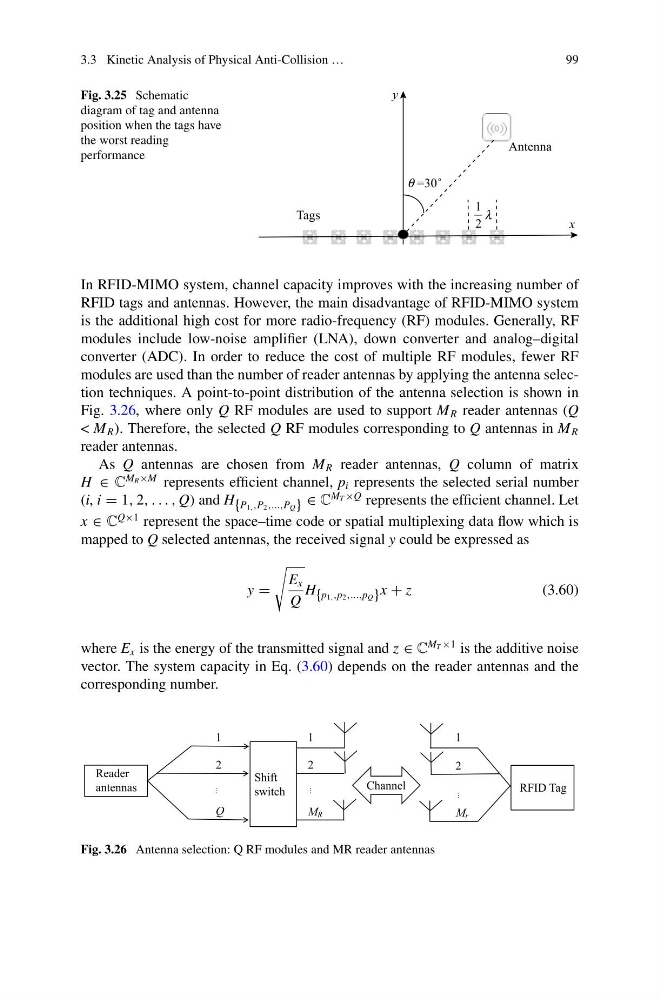
Fig. 3.25 Schematic
diagram of tag and antenna
position when the tags have
the worst reading
performance
In RFID-MIMO system, channel capacity improves with the increasing number of
RFID tags and antennas. However, the main disadvantage of RFID-MIMO system
is the additional high cost for more radio-frequency (RF) modules. Generally, RF
modules include low-noise amplifier (LNA), down converter and analog–digital
converter (ADC). In order to reduce the cost of multiple RF modules, fewer RF
modules are used than the number of reader antennas by applying the antenna selection techniques. A point-to-point distribution of the antenna selection is shown in
Fig. 3.26, where only Q RF modules are used to support M R reader antennas (Q
< M R ). Therefore, the selected Q RF modules corresponding to Q antennas in M R
reader antennas.
As Q antennas are chosen from M R reader antennas, Q column of matrix
H ∈ C
M R ×M represents efficient channel, p i represents the selected serial number
(i, i = 1, 2, . . . , Q) and H {P1,,P2,...,PQ} ∈ C
M T ×Q represents the efficient channel. Let
x ∈ C
Q×1 represent the space–time code or spatial multiplexing data flow which is
mapped to Q selected antennas, the received signal y could be expressed as
y =
E x
Q
H {p1,,p2,...,pQ} x + z
(3.60)
where E x is the energy of the transmitted signal and z ∈ C
M T ×1 is the additive noise
vector. The system capacity in Eq. (3.60) depends on the reader antennas and the
corresponding number.
Fig. 3.26 Antenna selection: Q RF modules and MR reader antennas
99
Fig. 3.25 Schematic
diagram of tag and antenna
position when the tags have
the worst reading
performance
In RFID-MIMO system, channel capacity improves with the increasing number of
RFID tags and antennas. However, the main disadvantage of RFID-MIMO system
is the additional high cost for more radio-frequency (RF) modules. Generally, RF
modules include low-noise amplifier (LNA), down converter and analog–digital
converter (ADC). In order to reduce the cost of multiple RF modules, fewer RF
modules are used than the number of reader antennas by applying the antenna selection techniques. A point-to-point distribution of the antenna selection is shown in
Fig. 3.26, where only Q RF modules are used to support M R reader antennas (Q
< M R ). Therefore, the selected Q RF modules corresponding to Q antennas in M R
reader antennas.
As Q antennas are chosen from M R reader antennas, Q column of matrix
H ∈ C
M R ×M represents efficient channel, p i represents the selected serial number
(i, i = 1, 2, . . . , Q) and H {P1,,P2,...,PQ} ∈ C
M T ×Q represents the efficient channel. Let
x ∈ C
Q×1 represent the space–time code or spatial multiplexing data flow which is
mapped to Q selected antennas, the received signal y could be expressed as
y =
E x
Q
H {p1,,p2,...,pQ} x + z
(3.60)
where E x is the energy of the transmitted signal and z ∈ C
M T ×1 is the additive noise
vector. The system capacity in Eq. (3.60) depends on the reader antennas and the
corresponding number.
Fig. 3.26 Antenna selection: Q RF modules and MR reader antennas