

Vibrations with Collisions of a Mechanical …
71
If the generic rigid body p collides the left stopper, then the previous expression
becomes
˙
x p (t + ) = −r p ˙
x p (t − ), with ˙
x p (t − ) < 0,
(14)
while the collision takes place with the right stopper, one may write
˙
x p (t + ) = −r p ˙
x p (t − ), with ˙
x p (t − ) > 0
(15)
3 Numerical Example
As a numerical example, we consider n = 3, m 1 = 1 kg, m 2 = 2 kg, m 3 = 3 kg,
y 1 = 0.1 m, y 2 = 0.25 m, y 3 = 0.3 m, k 1 = 20 N/m, k 2 = 10 N/m, k 3 = 15 N/m,
X 0 = 0.3 m, A 0 = 0.5 m, ω = 10 s
−1 , b 1s = 0.2 m, b 1d = 0.35 m, b 2s = 0.18 m,
b 2d = 0.4 m, b 3s = 0.15 m, b 3d = 0.5 m, x 10 = x 20 = x 30 = 0.3 m, ˙
x 10 = ˙
x 20 =
˙
x 30 = 0 m/s, r 1 = 0.6, r 2 = 0.7, r 3 = 0.9, number of iterations N = 50, 000, step
of iterations dt = 0.001 s.
Different other values are also selected for the parameters of the system: new
values for the positions of the stoppers, different values for the stiffness, the coefficients of restitution (including the values 0 (plastic collision) and 1 (elastic collision)),
positions of the horizontal bars, excitation. In all cases, the diagrams of variations
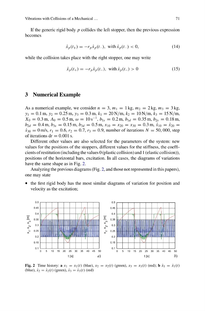
have the same shape as in Fig. 2.
Analyzing the previous diagrams (Fig. 2, and those not represented in this papers),
one may state
• the first rigid body has the most similar diagrams of variation for position and
velocity as the excitation;
a)
b)
0
5
10 15 20 25 30 35 40 45 50
0.1
0.15
0.2
0.25
0.3
0.35
0.4
0.45
0.5
t [s]
x
1
, x
2
, x
3
[m]
0
5
10 15 20 25 30 35 40 45 50
0.1
0.15
0.2
0.25
0.3
0.35
0.4
0.45
0.5
t [s]
x
1
, x
2
, x
3
[m]
Fig. 2 Time history: a x 1 = x 1 (t) (blue), x 2 = x 2 (t) (green), x 3 = x 3 (t) (red); b ˙
x 1 = ˙
x 1 (t)
(blue), ˙
x 2 = ˙
x 2 (t) (green), ˙
x 3 = ˙
x 3 (t) (red)
71
If the generic rigid body p collides the left stopper, then the previous expression
becomes
˙
x p (t + ) = −r p ˙
x p (t − ), with ˙
x p (t − ) < 0,
(14)
while the collision takes place with the right stopper, one may write
˙
x p (t + ) = −r p ˙
x p (t − ), with ˙
x p (t − ) > 0
(15)
3 Numerical Example
As a numerical example, we consider n = 3, m 1 = 1 kg, m 2 = 2 kg, m 3 = 3 kg,
y 1 = 0.1 m, y 2 = 0.25 m, y 3 = 0.3 m, k 1 = 20 N/m, k 2 = 10 N/m, k 3 = 15 N/m,
X 0 = 0.3 m, A 0 = 0.5 m, ω = 10 s
−1 , b 1s = 0.2 m, b 1d = 0.35 m, b 2s = 0.18 m,
b 2d = 0.4 m, b 3s = 0.15 m, b 3d = 0.5 m, x 10 = x 20 = x 30 = 0.3 m, ˙
x 10 = ˙
x 20 =
˙
x 30 = 0 m/s, r 1 = 0.6, r 2 = 0.7, r 3 = 0.9, number of iterations N = 50, 000, step
of iterations dt = 0.001 s.
Different other values are also selected for the parameters of the system: new
values for the positions of the stoppers, different values for the stiffness, the coefficients of restitution (including the values 0 (plastic collision) and 1 (elastic collision)),
positions of the horizontal bars, excitation. In all cases, the diagrams of variations
have the same shape as in Fig. 2.
Analyzing the previous diagrams (Fig. 2, and those not represented in this papers),
one may state
• the first rigid body has the most similar diagrams of variation for position and
velocity as the excitation;
a)
b)
0
5
10 15 20 25 30 35 40 45 50
0.1
0.15
0.2
0.25
0.3
0.35
0.4
0.45
0.5
t [s]
x
1
, x
2
, x
3
[m]
0
5
10 15 20 25 30 35 40 45 50
0.1
0.15
0.2
0.25
0.3
0.35
0.4
0.45
0.5
t [s]
x
1
, x
2
, x
3
[m]
Fig. 2 Time history: a x 1 = x 1 (t) (blue), x 2 = x 2 (t) (green), x 3 = x 3 (t) (red); b ˙
x 1 = ˙
x 1 (t)
(blue), ˙
x 2 = ˙
x 2 (t) (green), ˙
x 3 = ˙
x 3 (t) (red)