

Optimal Auxiliary Functions Method for Nonlinear Vibration …
55
3 Galerkin Formulation
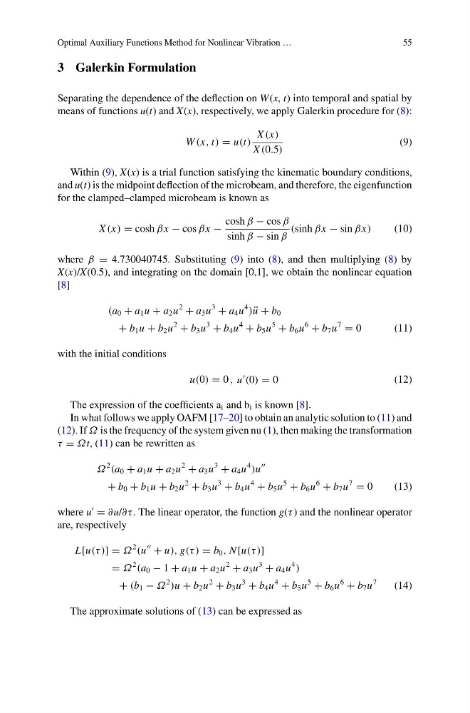
Separating the dependence of the deflection on W (x, t) into temporal and spatial by
means of functions u(t) and X(x), respectively, we apply Galerkin procedure for (8):
W (x, t) = u(t)
X (x)
X (0.5)
(9)
Within (9), X(x) is a trial function satisfying the kinematic boundary conditions,
and u(t) is the midpoint deflection of the microbeam, and therefore, the eigenfunction
for the clamped–clamped microbeam is known as
X (x) = cosh βx − cos βx −
cosh β − cos β
sinh β − sin β
(sinh βx − sin βx)
(10)
where β = 4.730040745. Substituting (9) into (8), and then multiplying (8) by
X(x)/X(0.5), and integrating on the domain [0,1], we obtain the nonlinear equation
[8]
(a 0 + a 1 u + a 2 u
2
+ a 3 u
3
+ a 4 u
4
) ¨
u + b 0
+ b 1 u + b 2 u
2
+ b 3 u
3
+ b 4 u
4
+ b 5 u
5
+ b 6 u
6
+ b 7 u
7
= 0
(11)
with the initial conditions
u(0) = 0 , u
(0) = 0
(12)
The expression of the coefficients a i and b i is known [8].
In what follows we apply OAFM [17–20] to obtain an analytic solution to (11) and
(12). If Ω is the frequency of the system given nu (1), then making the transformation
τ = Ωt, (11) can be rewritten as
Ω
2
(a 0 + a 1 u + a 2 u
2
+ a 3 u
3
+ a 4 u
4
)u
+ b 0 + b 1 u + b 2 u
2
+ b 3 u
3
+ b 4 u
4
+ b 5 u
5
+ b 6 u
6
+ b 7 u
7
= 0
(13)
where u
= ∂u/∂τ. The linear operator, the function g(τ ) and the nonlinear operator
are, respectively
L[u(τ )] = Ω
2
(u
+ u), g(τ ) = b 0 , N [u(τ )]
= Ω
2
(a 0 − 1 + a 1 u + a 2 u
2
+ a 3 u
3
+ a 4 u
4
)
+ (b 1 − Ω
2
)u + b 2 u
2
+ b 3 u
3
+ b 4 u
4
+ b 5 u
5
+ b 6 u
6
+ b 7 u
7
(14)
The approximate solutions of (13) can be expressed as
55
3 Galerkin Formulation
Separating the dependence of the deflection on W (x, t) into temporal and spatial by
means of functions u(t) and X(x), respectively, we apply Galerkin procedure for (8):
W (x, t) = u(t)
X (x)
X (0.5)
(9)
Within (9), X(x) is a trial function satisfying the kinematic boundary conditions,
and u(t) is the midpoint deflection of the microbeam, and therefore, the eigenfunction
for the clamped–clamped microbeam is known as
X (x) = cosh βx − cos βx −
cosh β − cos β
sinh β − sin β
(sinh βx − sin βx)
(10)
where β = 4.730040745. Substituting (9) into (8), and then multiplying (8) by
X(x)/X(0.5), and integrating on the domain [0,1], we obtain the nonlinear equation
[8]
(a 0 + a 1 u + a 2 u
2
+ a 3 u
3
+ a 4 u
4
) ¨
u + b 0
+ b 1 u + b 2 u
2
+ b 3 u
3
+ b 4 u
4
+ b 5 u
5
+ b 6 u
6
+ b 7 u
7
= 0
(11)
with the initial conditions
u(0) = 0 , u
(0) = 0
(12)
The expression of the coefficients a i and b i is known [8].
In what follows we apply OAFM [17–20] to obtain an analytic solution to (11) and
(12). If Ω is the frequency of the system given nu (1), then making the transformation
τ = Ωt, (11) can be rewritten as
Ω
2
(a 0 + a 1 u + a 2 u
2
+ a 3 u
3
+ a 4 u
4
)u
+ b 0 + b 1 u + b 2 u
2
+ b 3 u
3
+ b 4 u
4
+ b 5 u
5
+ b 6 u
6
+ b 7 u
7
= 0
(13)
where u
= ∂u/∂τ. The linear operator, the function g(τ ) and the nonlinear operator
are, respectively
L[u(τ )] = Ω
2
(u
+ u), g(τ ) = b 0 , N [u(τ )]
= Ω
2
(a 0 − 1 + a 1 u + a 2 u
2
+ a 3 u
3
+ a 4 u
4
)
+ (b 1 − Ω
2
)u + b 2 u
2
+ b 3 u
3
+ b 4 u
4
+ b 5 u
5
+ b 6 u
6
+ b 7 u
7
(14)
The approximate solutions of (13) can be expressed as