

Improved Model of a Vibrating Sieve
399
[I ] − Ω
2 [D]
{A} + μΩ[I ]{B} = { f 0 }
−μΩ[I ]{A} +
[I ] − Ω
2 [D]
{B} = {0}
,
(19)
[I ] − Ω
2 [D]
μΩ[I ]
−μΩ[I ] [I ] − Ω
2 [D]
{A}
{B}
=
{ f 0 }
{0}
.
(20)
By solving the above algebraic system, vectors {A}, {B} are obtained.
3 Numerical Analysis
For the numerical application, the following values were considered: the mass of the
sieve m s = 3902 kg, the mass of the sieve with excitator 5105 kg, the length of the
blades 45 cm long, Young’s modulus E = 2.1 · 10
11 N/m
2 and the moment of inertia
of the cross-section I = 2 · I 0 = 2 ·
b·h
3
12
where b = 60 mm and h = 2 mm.
Two values were considered for the damping: ˜
x = 0.01 and ˜
x = 0.02, and three
positions for the excitator: 1 on the lower sieve, 2 on the middle sieve and 3 on the
top sieve.
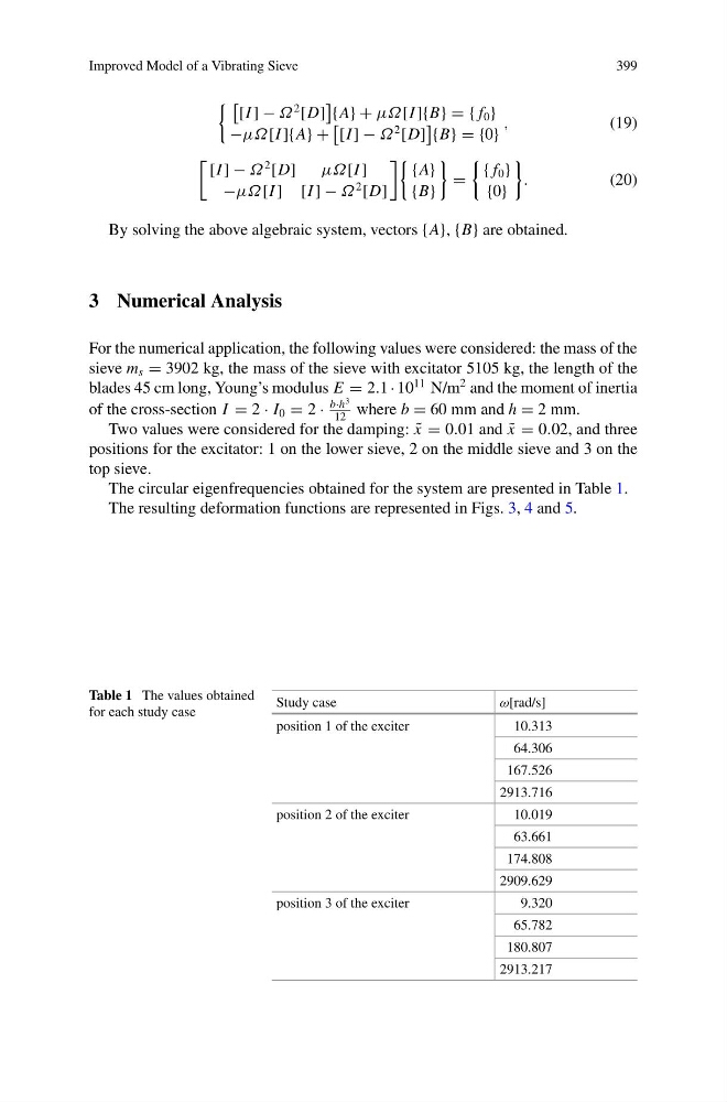
The circular eigenfrequencies obtained for the system are presented in Table 1.
The resulting deformation functions are represented in Figs. 3, 4 and 5.
Table 1 The values obtained
for each study case
Study case
ω[rad/s]
position 1 of the exciter
10.313
64.306
167.526
2913.716
position 2 of the exciter
10.019
63.661
174.808
2909.629
position 3 of the exciter
9.320
65.782
180.807
2913.217
399
[I ] − Ω
2 [D]
{A} + μΩ[I ]{B} = { f 0 }
−μΩ[I ]{A} +
[I ] − Ω
2 [D]
{B} = {0}
,
(19)
[I ] − Ω
2 [D]
μΩ[I ]
−μΩ[I ] [I ] − Ω
2 [D]
{A}
{B}
=
{ f 0 }
{0}
.
(20)
By solving the above algebraic system, vectors {A}, {B} are obtained.
3 Numerical Analysis
For the numerical application, the following values were considered: the mass of the
sieve m s = 3902 kg, the mass of the sieve with excitator 5105 kg, the length of the
blades 45 cm long, Young’s modulus E = 2.1 · 10
11 N/m
2 and the moment of inertia
of the cross-section I = 2 · I 0 = 2 ·
b·h
3
12
where b = 60 mm and h = 2 mm.
Two values were considered for the damping: ˜
x = 0.01 and ˜
x = 0.02, and three
positions for the excitator: 1 on the lower sieve, 2 on the middle sieve and 3 on the
top sieve.
The circular eigenfrequencies obtained for the system are presented in Table 1.
The resulting deformation functions are represented in Figs. 3, 4 and 5.
Table 1 The values obtained
for each study case
Study case
ω[rad/s]
position 1 of the exciter
10.313
64.306
167.526
2913.716
position 2 of the exciter
10.019
63.661
174.808
2909.629
position 3 of the exciter
9.320
65.782
180.807
2913.217