

Parametric Analysis of Dynamic Insulation in the Action …
369
2 Dynamic Response
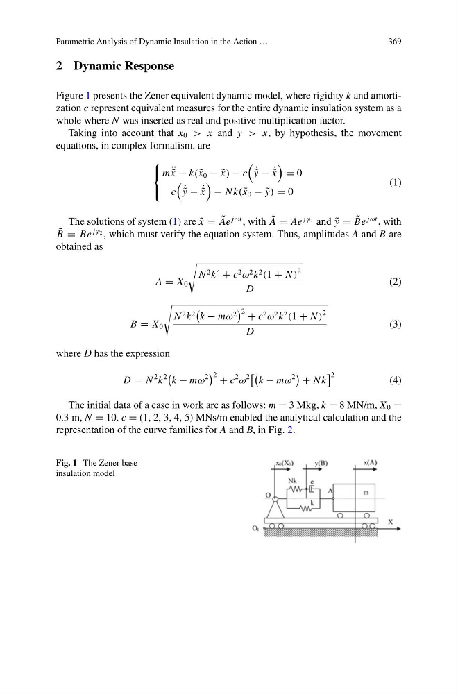
Figure 1 presents the Zener equivalent dynamic model, where rigidity k and amortization c represent equivalent measures for the entire dynamic insulation system as a
whole where N was inserted as real and positive multiplication factor.
Taking into account that x 0 > x and y > x, by hypothesis, the movement
equations, in complex formalism, are
⎧
⎨
⎩
m ¨ ˜
x − k( ˜
x 0 − ˜
x) − c
˙ ˜
y − ˙ ˜
x
= 0
c
˙ ˜
y − ˙ ˜
x
− N k( ˜
x 0 − ˜
y) = 0
(1)
The solutions of system (1) are ˜
x = ˜
Ae
jωt , with ˜
A = Ae
jϕ 1 and ˜
y = ˜
Be
jωt , with
˜
B = Be
jϕ 2 , which must verify the equation system. Thus, amplitudes A and B are
obtained as
A = X 0
N 2 k 4 + c 2 ω 2 k 2 (1 + N )
2
D
(2)
B = X 0
N 2 k 2
k − mω 2
2 + c 2 ω 2 k 2 (1 + N )
2
D
(3)
where D has the expression
D = N
2 k
2
k − mω
2
2 + c
2
ω
2
k − mω
2
+ N k
2
(4)
The initial data of a case in work are as follows: m = 3 Mkg, k = 8 MN/m, X 0 =
0.3 m, N = 10. c = (1, 2, 3, 4, 5) MNs/m enabled the analytical calculation and the
representation of the curve families for A and B, in Fig. 2.
Fig. 1 The Zener base
insulation model
369
2 Dynamic Response
Figure 1 presents the Zener equivalent dynamic model, where rigidity k and amortization c represent equivalent measures for the entire dynamic insulation system as a
whole where N was inserted as real and positive multiplication factor.
Taking into account that x 0 > x and y > x, by hypothesis, the movement
equations, in complex formalism, are
⎧
⎨
⎩
m ¨ ˜
x − k( ˜
x 0 − ˜
x) − c
˙ ˜
y − ˙ ˜
x
= 0
c
˙ ˜
y − ˙ ˜
x
− N k( ˜
x 0 − ˜
y) = 0
(1)
The solutions of system (1) are ˜
x = ˜
Ae
jωt , with ˜
A = Ae
jϕ 1 and ˜
y = ˜
Be
jωt , with
˜
B = Be
jϕ 2 , which must verify the equation system. Thus, amplitudes A and B are
obtained as
A = X 0
N 2 k 4 + c 2 ω 2 k 2 (1 + N )
2
D
(2)
B = X 0
N 2 k 2
k − mω 2
2 + c 2 ω 2 k 2 (1 + N )
2
D
(3)
where D has the expression
D = N
2 k
2
k − mω
2
2 + c
2
ω
2
k − mω
2
+ N k
2
(4)
The initial data of a case in work are as follows: m = 3 Mkg, k = 8 MN/m, X 0 =
0.3 m, N = 10. c = (1, 2, 3, 4, 5) MNs/m enabled the analytical calculation and the
representation of the curve families for A and B, in Fig. 2.
Fig. 1 The Zener base
insulation model