

Gears Dynamic Response to Vibrations
93
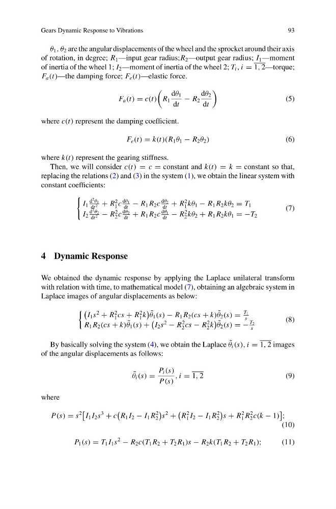
θ 1 , θ 2 are the angular displacements of the wheel and the sprocket around their axis
of rotation, in degree; R 1 —input gear radius;R 2 —output gear radius; I 1 —moment
of inertia of the wheel 1; I 2 —moment of inertia of the wheel 2; T i , i = 1, 2—torque;
F a (t)—the damping force; F e (t)—elastic force.
F a (t) = c(t)
R 1
dθ 1
dt
− R 2
dθ 2
dt
(5)
where c(t) represent the damping coefficient.
F e (t) = k(t)(R 1 θ 1 − R 2 θ 2 )
(6)
where k(t) represent the gearing stiffness.
Then, we will consider c(t) = c = constant and k(t) = k = constant so that,
replacing the relations (2) and (3) in the system (1), we obtain the linear system with
constant coefficients:
I 1
d
2 θ 1
dt 2 + R
2
1 c
dθ 1
dt
− R 1 R 2 c
dθ 2
dt
+ R
2
1 kθ 1 − R 1 R 2 kθ 2 = T 1
I 2
d
2 θ 2
dt 2 − R
2
2 c
dθ 2
dt
+ R 1 R 2 c
dθ 1
dt
− R
2
2 kθ 2 + R 1 R 2 kθ 1 = −T 2
(7)
4 Dynamic Response
We obtained the dynamic response by applying the Laplace unilateral transform
with relation with time, to mathematical model (7), obtaining an algebraic system in
Laplace images of angular displacements as below:
I 1 s
2
+ R
2
1 cs + R
2
1 k
˜
θ 1 (s) − R 1 R 2 (cs + k) ˜
θ 2 (s) =
T 1
s
R 1 R 2 (cs + k) ˜
θ 1 (s) +
I 2 s
2
− R
2
2 cs − R
2
2 k
˜
θ 2 (s) = −
T 2
s
(8)
By basically solving the system (4), we obtain the Laplace ˜
θ i (s), i = 1, 2 images
of the angular displacements as follows:
˜
θ i (s) =
P i (s)
P(s)
, i = 1, 2
( 9 )
where
P(s) = s
2
I 1 I 2 s
3
+ c
R 1 I 2 − I 1 R
2
2
s
2
+
R
2
1 I 2 − I 1 R
2
2
s + R
2
1 R
2
2 c(k − 1)
;
(10)
P 1 (s) = T 1 I 1 s
2
− R 2 c(T 1 R 2 + T 2 R 1 )s − R 2 k(T 1 R 2 + T 2 R 1 );
(11)
93
θ 1 , θ 2 are the angular displacements of the wheel and the sprocket around their axis
of rotation, in degree; R 1 —input gear radius;R 2 —output gear radius; I 1 —moment
of inertia of the wheel 1; I 2 —moment of inertia of the wheel 2; T i , i = 1, 2—torque;
F a (t)—the damping force; F e (t)—elastic force.
F a (t) = c(t)
R 1
dθ 1
dt
− R 2
dθ 2
dt
(5)
where c(t) represent the damping coefficient.
F e (t) = k(t)(R 1 θ 1 − R 2 θ 2 )
(6)
where k(t) represent the gearing stiffness.
Then, we will consider c(t) = c = constant and k(t) = k = constant so that,
replacing the relations (2) and (3) in the system (1), we obtain the linear system with
constant coefficients:
I 1
d
2 θ 1
dt 2 + R
2
1 c
dθ 1
dt
− R 1 R 2 c
dθ 2
dt
+ R
2
1 kθ 1 − R 1 R 2 kθ 2 = T 1
I 2
d
2 θ 2
dt 2 − R
2
2 c
dθ 2
dt
+ R 1 R 2 c
dθ 1
dt
− R
2
2 kθ 2 + R 1 R 2 kθ 1 = −T 2
(7)
4 Dynamic Response
We obtained the dynamic response by applying the Laplace unilateral transform
with relation with time, to mathematical model (7), obtaining an algebraic system in
Laplace images of angular displacements as below:
I 1 s
2
+ R
2
1 cs + R
2
1 k
˜
θ 1 (s) − R 1 R 2 (cs + k) ˜
θ 2 (s) =
T 1
s
R 1 R 2 (cs + k) ˜
θ 1 (s) +
I 2 s
2
− R
2
2 cs − R
2
2 k
˜
θ 2 (s) = −
T 2
s
(8)
By basically solving the system (4), we obtain the Laplace ˜
θ i (s), i = 1, 2 images
of the angular displacements as follows:
˜
θ i (s) =
P i (s)
P(s)
, i = 1, 2
( 9 )
where
P(s) = s
2
I 1 I 2 s
3
+ c
R 1 I 2 − I 1 R
2
2
s
2
+
R
2
1 I 2 − I 1 R
2
2
s + R
2
1 R
2
2 c(k − 1)
;
(10)
P 1 (s) = T 1 I 1 s
2
− R 2 c(T 1 R 2 + T 2 R 1 )s − R 2 k(T 1 R 2 + T 2 R 1 );
(11)