

92
V. Ionica et al.
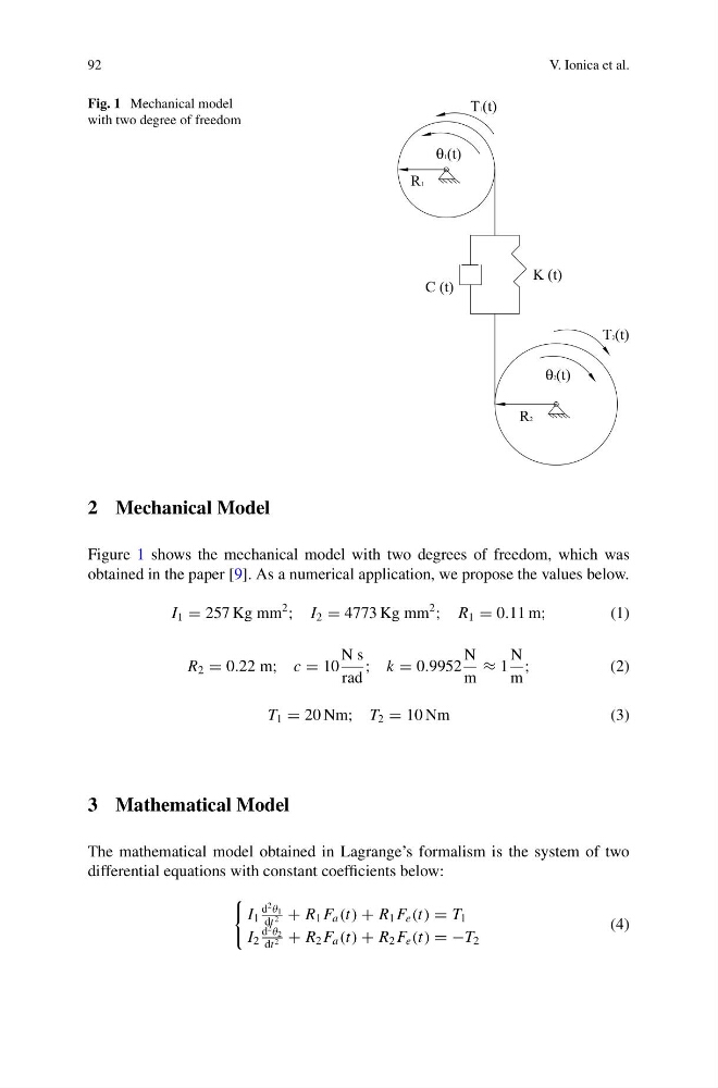
Fig. 1 Mechanical model
with two degree of freedom
θ1(t)
θ2(t)
C (t)
K (t)
T1(t)
T2(t)
R1
R2
2 Mechanical Model
Figure 1 shows the mechanical model with two degrees of freedom, which was
obtained in the paper [9]. As a numerical application, we propose the values below.
I 1 = 257 Kg mm
2
; I 2 = 4773 Kg mm
2
; R 1 = 0.11 m;
(1)
R 2 = 0.22 m; c = 10
N s
rad
; k = 0.9952
N
m
≈ 1
N
m
;
(2)
T 1 = 20 Nm; T 2 = 10 Nm
(3)
3 Mathematical Model
The mathematical model obtained in Lagrange’s formalism is the system of two
differential equations with constant coefficients below:
I 1
d
2 θ 1
dt 2 + R 1 F a (t) + R 1 F e (t) = T 1
I 2
d
2 θ 2
dt 2 + R 2 F a (t) + R 2 F e (t) = −T 2
(4)
V. Ionica et al.
Fig. 1 Mechanical model
with two degree of freedom
θ1(t)
θ2(t)
C (t)
K (t)
T1(t)
T2(t)
R1
R2
2 Mechanical Model
Figure 1 shows the mechanical model with two degrees of freedom, which was
obtained in the paper [9]. As a numerical application, we propose the values below.
I 1 = 257 Kg mm
2
; I 2 = 4773 Kg mm
2
; R 1 = 0.11 m;
(1)
R 2 = 0.22 m; c = 10
N s
rad
; k = 0.9952
N
m
≈ 1
N
m
;
(2)
T 1 = 20 Nm; T 2 = 10 Nm
(3)
3 Mathematical Model
The mathematical model obtained in Lagrange’s formalism is the system of two
differential equations with constant coefficients below:
I 1
d
2 θ 1
dt 2 + R 1 F a (t) + R 1 F e (t) = T 1
I 2
d
2 θ 2
dt 2 + R 2 F a (t) + R 2 F e (t) = −T 2
(4)