

106 The Bennett linkage
Because FM // GI and FG // MI, we have
,
(5.76)
,
(5.77)
and F′M′ ⊥ W′U′. Then,
,
(5.78)
and
.
(5.79)
Substituting Eqs (5.74), (5.76) and (5.79) into (5.75), there is
.
(5.80)
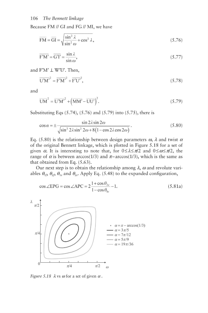
Eq. (5.80) is the relationship between design parameters ω, λ and twist α
of the original Bennett linkage, which is plotted in Figure 5.18 for a set of
given α. It is interesting to note that, for 0 ≤ λ ≤ π/2 and 0 ≤ ω ≤ π/2, the
range of α is between arccos(1/3) and π – arccos(1/3), which is the same as
that obtained from Eq. (5.63).
Our next step is to obtain the relationship among λ, ω and revolute variables θ 1f , θ 2f , θ 1e and θ 2e . Apply Eq. (5.48) to the expanded configuration,
.
(5.81a)
Figure 5.18 λ vs ω for a set of given α .
Because FM // GI and FG // MI, we have
,
(5.76)
,
(5.77)
and F′M′ ⊥ W′U′. Then,
,
(5.78)
and
.
(5.79)
Substituting Eqs (5.74), (5.76) and (5.79) into (5.75), there is
.
(5.80)
Eq. (5.80) is the relationship between design parameters ω, λ and twist α
of the original Bennett linkage, which is plotted in Figure 5.18 for a set of
given α. It is interesting to note that, for 0 ≤ λ ≤ π/2 and 0 ≤ ω ≤ π/2, the
range of α is between arccos(1/3) and π – arccos(1/3), which is the same as
that obtained from Eq. (5.63).
Our next step is to obtain the relationship among λ, ω and revolute variables θ 1f , θ 2f , θ 1e and θ 2e . Apply Eq. (5.48) to the expanded configuration,
.
(5.81a)
Figure 5.18 λ vs ω for a set of given α .