

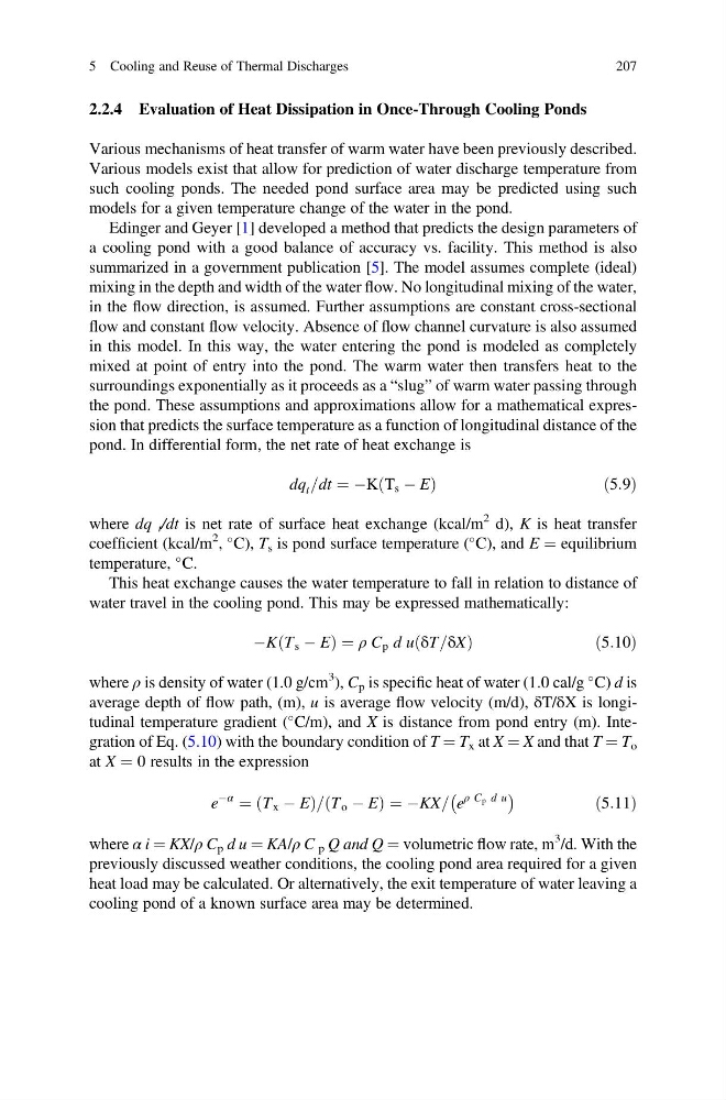
2.2.4 Evaluation of Heat Dissipation in Once-Through Cooling Ponds
Various mechanisms of heat transfer of warm water have been previously described.
Various models exist that allow for prediction of water discharge temperature from
such cooling ponds. The needed pond surface area may be predicted using such
models for a given temperature change of the water in the pond.
Edinger and Geyer [1] developed a method that predicts the design parameters of
a cooling pond with a good balance of accuracy vs. facility. This method is also
summarized in a government publication [5]. The model assumes complete (ideal)
mixing in the depth and width of the water flow. No longitudinal mixing of the water,
in the flow direction, is assumed. Further assumptions are constant cross-sectional
flow and constant flow velocity. Absence of flow channel curvature is also assumed
in this model. In this way, the water entering the pond is modeled as completely
mixed at point of entry into the pond. The warm water then transfers heat to the
surroundings exponentially as it proceeds as a “slug” of warm water passing through
the pond. These assumptions and approximations allow for a mathematical expression that predicts the surface temperature as a function of longitudinal distance of the
pond. In differential form, the net rate of heat exchange is
dq t =dt ¼ ÀK T s À E
ð
Þ
ð5:9Þ
where dq t /dt is net rate of surface heat exchange (kcal/m
2 d), K is heat transfer
coefficient (kcal/m
2 ,
C), T s is pond surface temperature (
C), and E ¼ equilibrium
temperature,
C.
This heat exchange causes the water temperature to fall in relation to distance of
water travel in the cooling pond. This may be expressed mathematically:
ÀK T s À E
ð
Þ¼ρ C p d u δT=δX
ð
Þ
ð5:10Þ
where ρ is density of water (1.0 g/cm
3 ), C p is specific heat of water (1.0 cal/g
C) d is
average depth of flow path, (m), u is average flow velocity (m/d), δT/δX is longitudinal temperature gradient (
C/m), and X is distance from pond entry (m). Integration of Eq. (5.10) with the boundary condition of T ¼ T x at X ¼ X and that T ¼ T o
at X ¼ 0 results in the expression
e
Àα
¼ T x À E
ð
Þ= T o À E
ð
Þ¼ÀKX= e
ρ C p d u
À
Á
ð5:11Þ
where α i ¼ KX/ρ C p d u ¼ KA/ρ C p Q and Q ¼ volumetric flow rate, m
3 /d. With the
previously discussed weather conditions, the cooling pond area required for a given
heat load may be calculated. Or alternatively, the exit temperature of water leaving a
cooling pond of a known surface area may be determined.
5 Cooling and Reuse of Thermal Discharges
207
Various mechanisms of heat transfer of warm water have been previously described.
Various models exist that allow for prediction of water discharge temperature from
such cooling ponds. The needed pond surface area may be predicted using such
models for a given temperature change of the water in the pond.
Edinger and Geyer [1] developed a method that predicts the design parameters of
a cooling pond with a good balance of accuracy vs. facility. This method is also
summarized in a government publication [5]. The model assumes complete (ideal)
mixing in the depth and width of the water flow. No longitudinal mixing of the water,
in the flow direction, is assumed. Further assumptions are constant cross-sectional
flow and constant flow velocity. Absence of flow channel curvature is also assumed
in this model. In this way, the water entering the pond is modeled as completely
mixed at point of entry into the pond. The warm water then transfers heat to the
surroundings exponentially as it proceeds as a “slug” of warm water passing through
the pond. These assumptions and approximations allow for a mathematical expression that predicts the surface temperature as a function of longitudinal distance of the
pond. In differential form, the net rate of heat exchange is
dq t =dt ¼ ÀK T s À E
ð
Þ
ð5:9Þ
where dq t /dt is net rate of surface heat exchange (kcal/m
2 d), K is heat transfer
coefficient (kcal/m
2 ,
C), T s is pond surface temperature (
C), and E ¼ equilibrium
temperature,
C.
This heat exchange causes the water temperature to fall in relation to distance of
water travel in the cooling pond. This may be expressed mathematically:
ÀK T s À E
ð
Þ¼ρ C p d u δT=δX
ð
Þ
ð5:10Þ
where ρ is density of water (1.0 g/cm
3 ), C p is specific heat of water (1.0 cal/g
C) d is
average depth of flow path, (m), u is average flow velocity (m/d), δT/δX is longitudinal temperature gradient (
C/m), and X is distance from pond entry (m). Integration of Eq. (5.10) with the boundary condition of T ¼ T x at X ¼ X and that T ¼ T o
at X ¼ 0 results in the expression
e
Àα
¼ T x À E
ð
Þ= T o À E
ð
Þ¼ÀKX= e
ρ C p d u
À
Á
ð5:11Þ
where α i ¼ KX/ρ C p d u ¼ KA/ρ C p Q and Q ¼ volumetric flow rate, m
3 /d. With the
previously discussed weather conditions, the cooling pond area required for a given
heat load may be calculated. Or alternatively, the exit temperature of water leaving a
cooling pond of a known surface area may be determined.
5 Cooling and Reuse of Thermal Discharges
207