

246
C. Binns et al.
S z +
7
2
T z =
L s
μ ↑↑ (ω) − μ ↑↓ (ω)
dω − 2
L 2
μ ↑↑ (ω) − μ ↑↓ (ω)
dω
L 2 +L s
μ ↑↑ (ω) + μ ↑↓ (ω)
dω
n h
(10.5)
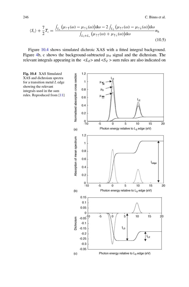
Figure 10.4 shows simulated dichroic XAS with a fitted integral background.
Figure 4b, c shows the background-subtracted μ 0 signal and the dichroism. The
relevant integrals appearing in the and sum rules are also indicated on
Fig. 10.4 XAS Simulated
XAS and dichroism spectra
for a transition metal L edge
showing the relevant
integrals used in the sum
rules. Reproduced from [11]
C. Binns et al.
S z +
7
2
T z =
L s
μ ↑↑ (ω) − μ ↑↓ (ω)
dω − 2
L 2
μ ↑↑ (ω) − μ ↑↓ (ω)
dω
L 2 +L s
μ ↑↑ (ω) + μ ↑↓ (ω)
dω
n h
(10.5)
Figure 10.4 shows simulated dichroic XAS with a fitted integral background.
Figure 4b, c shows the background-subtracted μ 0 signal and the dichroism. The
relevant integrals appearing in the
Fig. 10.4 XAS Simulated
XAS and dichroism spectra
for a transition metal L edge
showing the relevant
integrals used in the sum
rules. Reproduced from [11]