

1 Single Nanomagnet Behaviour: Surface and Finite-Size Effects
7
model and the corresponding Hamiltonian must necessarily make use of the atomic
magnetic moment as its elementary building block. Consequently, the techniques
for computing the various physical observables using such a Hamiltonian, generally
borrowed from bulk systems, have to be adapted and extended to such nano-scaled
systems, namely spin-wave theory, relaxation time theories, and Monte Carlo simulations, just to cite a few. In some limit, depending on the set of physical parameters,
it is possible to investigate the magnetization reversal of a NM within an assembly using a macroscopic model which represents the NM through its net magnetic
moment. Obviously, this model ignores any internal features of the NM and focuses
on its global behaviour in an external magnetic field and/or in contact with a heat
bath. There are several variants of such a model but all of them may be considered as
extensions of the initial Stoner-Wohlfarth (SW) and/or the Néel-Brown (NB) models
[4–10]. Up to scaling factors, these models are all one-spin problems and will then be
referred to as OSP. On the other hand, many-spin problems which involve the atomic
spins of the NM will be referred to as MSP. In this section we shall first succinctly
present the macroscopic model (OSP) and the well known results they render for the
magnetic moment of a NM under the usual conditions of temperature and magnetic
field. Next, we will turn to the presentation of the MSP approach, the corresponding
Hamiltonian and computational methods. In the subsequent sections, we will present
the main results of the application of this approach to a NM, regarded as a many-spin
crystal with its specific features.
1.2.1 Macrospin Approach
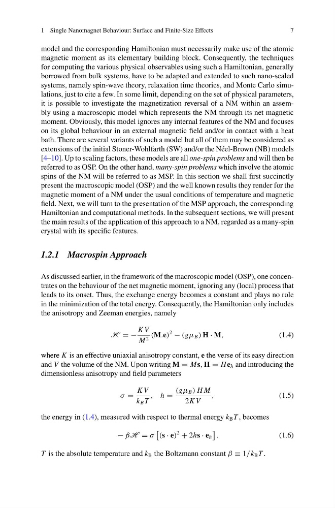
As discussed earlier, in the framework of the macroscopic model (OSP), one concentrates on the behaviour of the net magnetic moment, ignoring any (local) process that
leads to its onset. Thus, the exchange energy becomes a constant and plays no role
in the minimization of the total energy. Consequently, the Hamiltonian only includes
the anisotropy and Zeeman energies, namely
H = −
K V
M 2 (M.e)
2
− (gμ B ) H · M,
(1.4)
where K is an effective uniaxial anisotropy constant, e the verse of its easy direction
and V the volume of the NM. Upon writing M = Ms, H = H e h and introducing the
dimensionless anisotropy and field parameters
σ =
K V
k B T
, h =
(gμ B ) H M
2K V
,
(1.5)
the energy in (1.4), measured with respect to thermal energy k B T , becomes
− βH = σ
(s · e)
2
+ 2hs · e h
.
(1.6)
T is the absolute temperature and k B the Boltzmann constant β ≡ 1/k B T .
7
model and the corresponding Hamiltonian must necessarily make use of the atomic
magnetic moment as its elementary building block. Consequently, the techniques
for computing the various physical observables using such a Hamiltonian, generally
borrowed from bulk systems, have to be adapted and extended to such nano-scaled
systems, namely spin-wave theory, relaxation time theories, and Monte Carlo simulations, just to cite a few. In some limit, depending on the set of physical parameters,
it is possible to investigate the magnetization reversal of a NM within an assembly using a macroscopic model which represents the NM through its net magnetic
moment. Obviously, this model ignores any internal features of the NM and focuses
on its global behaviour in an external magnetic field and/or in contact with a heat
bath. There are several variants of such a model but all of them may be considered as
extensions of the initial Stoner-Wohlfarth (SW) and/or the Néel-Brown (NB) models
[4–10]. Up to scaling factors, these models are all one-spin problems and will then be
referred to as OSP. On the other hand, many-spin problems which involve the atomic
spins of the NM will be referred to as MSP. In this section we shall first succinctly
present the macroscopic model (OSP) and the well known results they render for the
magnetic moment of a NM under the usual conditions of temperature and magnetic
field. Next, we will turn to the presentation of the MSP approach, the corresponding
Hamiltonian and computational methods. In the subsequent sections, we will present
the main results of the application of this approach to a NM, regarded as a many-spin
crystal with its specific features.
1.2.1 Macrospin Approach
As discussed earlier, in the framework of the macroscopic model (OSP), one concentrates on the behaviour of the net magnetic moment, ignoring any (local) process that
leads to its onset. Thus, the exchange energy becomes a constant and plays no role
in the minimization of the total energy. Consequently, the Hamiltonian only includes
the anisotropy and Zeeman energies, namely
H = −
K V
M 2 (M.e)
2
− (gμ B ) H · M,
(1.4)
where K is an effective uniaxial anisotropy constant, e the verse of its easy direction
and V the volume of the NM. Upon writing M = Ms, H = H e h and introducing the
dimensionless anisotropy and field parameters
σ =
K V
k B T
, h =
(gμ B ) H M
2K V
,
(1.5)
the energy in (1.4), measured with respect to thermal energy k B T , becomes
− βH = σ
(s · e)
2
+ 2hs · e h
.
(1.6)
T is the absolute temperature and k B the Boltzmann constant β ≡ 1/k B T .