

2.4 Critical Mass: Tamped Composite Core
79
The various quantities appearing in these expressions are
(x 1 , x 2 , x 3 ) =
R 1
d 1
,
R 1
d 2
,
R 2
d 2
,
(2.72)
B
C
=
[δ Y sin x 1 + Z cos x 2 ]
[δ W sin x 1 − Z sin x 2 ]
,
(2.73)
and
ψ = −
λ
tran
2 d 2
λ
tran
tamp
,
(2.74)
with
W = [− sin x 2 + x 2 cos x 2 ],
(2.75)
Y = [cos x 2 + x 2 sin x 2 ],
(2.76)
Z = λ[− sin x 1 + x 1 cos x 1 ],
(2.77)
where
λ =
λ
tran
1
λ
tran
2
d 1
d 2
=
λ
tran
1
λ
tran
2
δ.
(2.78)
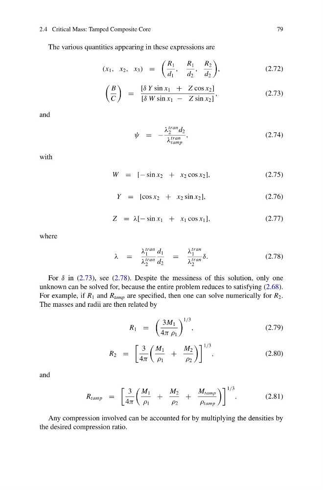
For δ in (2.73), see (2.78). Despite the messiness of this solution, only one
unknown can be solved for, because the entire problem reduces to satisfying (2.68).
For example, if R 1 and R tamp are specified, then one can solve numerically for R 2 .
The masses and radii are then related by
R 1 =
3M 1
4π ρ 1
1/3
,
(2.79)
R 2 =
3
4π
M 1
ρ 1
+
M 2
ρ 2
1/3
,
(2.80)
and
R tamp =
3
4π
M 1
ρ 1
+
M 2
ρ 2
+
M tamp
ρ tamp
1/3
.
(2.81)
Any compression involved can be accounted for by multiplying the densities by
the desired compression ratio.
79
The various quantities appearing in these expressions are
(x 1 , x 2 , x 3 ) =
R 1
d 1
,
R 1
d 2
,
R 2
d 2
,
(2.72)
B
C
=
[δ Y sin x 1 + Z cos x 2 ]
[δ W sin x 1 − Z sin x 2 ]
,
(2.73)
and
ψ = −
λ
tran
2 d 2
λ
tran
tamp
,
(2.74)
with
W = [− sin x 2 + x 2 cos x 2 ],
(2.75)
Y = [cos x 2 + x 2 sin x 2 ],
(2.76)
Z = λ[− sin x 1 + x 1 cos x 1 ],
(2.77)
where
λ =
λ
tran
1
λ
tran
2
d 1
d 2
=
λ
tran
1
λ
tran
2
δ.
(2.78)
For δ in (2.73), see (2.78). Despite the messiness of this solution, only one
unknown can be solved for, because the entire problem reduces to satisfying (2.68).
For example, if R 1 and R tamp are specified, then one can solve numerically for R 2 .
The masses and radii are then related by
R 1 =
3M 1
4π ρ 1
1/3
,
(2.79)
R 2 =
3
4π
M 1
ρ 1
+
M 2
ρ 2
1/3
,
(2.80)
and
R tamp =
3
4π
M 1
ρ 1
+
M 2
ρ 2
+
M tamp
ρ tamp
1/3
.
(2.81)
Any compression involved can be accounted for by multiplying the densities by
the desired compression ratio.