

200
6 Appendices
6.5.2 Nuclear Surface Profile and Volume
Bohr and Wheeler began by imagining an initially spherical nucleus of radius R O
undergoing a distortion expressible in the form
r (θ ) = R O {(1 + α 0 )P 0 (cos θ ) + α 2 P 2 (cos θ ) + · · ·}.
(6.25)
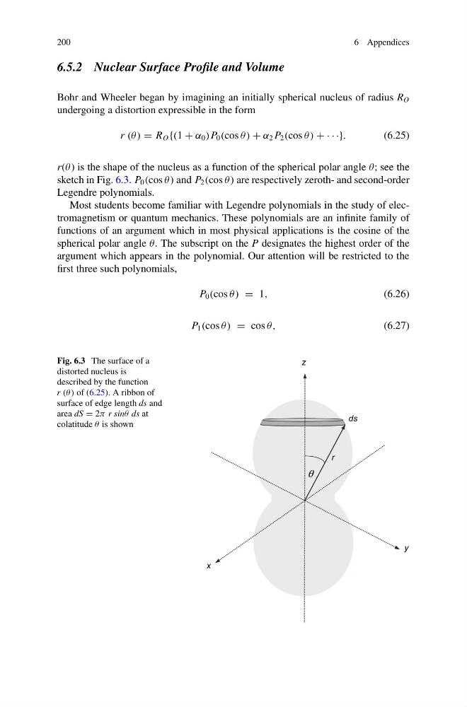
r(θ ) is the shape of the nucleus as a function of the spherical polar angle θ; see the
sketch in Fig. 6.3. P 0 (cos θ ) and P 2 (cos θ ) are respectively zeroth- and second-order
Legendre polynomials.
Most students become familiar with Legendre polynomials in the study of electromagnetism or quantum mechanics. These polynomials are an infinite family of
functions of an argument which in most physical applications is the cosine of the
spherical polar angle θ. The subscript on the P designates the highest order of the
argument which appears in the polynomial. Our attention will be restricted to the
first three such polynomials,
P 0 (cos θ ) = 1,
(6.26)
P 1 (cos θ ) = cos θ,
(6.27)
Fig. 6.3 The surface of a
distorted nucleus is
described by the function
r (θ) of (6.25). A ribbon of
surface of edge length ds and
area dS = 2π r sinθ ds at
colatitude θ is shown
z
y
x
r
θ
ds
6 Appendices
6.5.2 Nuclear Surface Profile and Volume
Bohr and Wheeler began by imagining an initially spherical nucleus of radius R O
undergoing a distortion expressible in the form
r (θ ) = R O {(1 + α 0 )P 0 (cos θ ) + α 2 P 2 (cos θ ) + · · ·}.
(6.25)
r(θ ) is the shape of the nucleus as a function of the spherical polar angle θ; see the
sketch in Fig. 6.3. P 0 (cos θ ) and P 2 (cos θ ) are respectively zeroth- and second-order
Legendre polynomials.
Most students become familiar with Legendre polynomials in the study of electromagnetism or quantum mechanics. These polynomials are an infinite family of
functions of an argument which in most physical applications is the cosine of the
spherical polar angle θ. The subscript on the P designates the highest order of the
argument which appears in the polynomial. Our attention will be restricted to the
first three such polynomials,
P 0 (cos θ ) = 1,
(6.26)
P 1 (cos θ ) = cos θ,
(6.27)
Fig. 6.3 The surface of a
distorted nucleus is
described by the function
r (θ) of (6.25). A ribbon of
surface of edge length ds and
area dS = 2π r sinθ ds at
colatitude θ is shown
z
y
x
r
θ
ds