

Chapitre 8 • La programmation linéaire
350
x 1
x 1
x 1
z
x 2
x 2
x 3
x 3 Primal
Dual
x 1
x 2
x 3
x 4
y 2
y 3
y 4
y 2
y 1
y 4
y 1
y 3
y 2
y 3
z
1/ 3
4/ 3
1/ 3
1/ 3
2/ 3
4/ 3
2/ 3
1/ 3
1/ 3
4
2
2
2
2
4
1
1500
1500
750
750
500
500
250
250
11500
11500
1
1/ 3
2/ 3
2/ 3
0
0
0
0
0
0
0
0
0
0
0
0
0
0
0
0
0
0
0
0
0
0
0
0
0
0
0
0
0
0
0
0
0
1
1
1
1
1
1
1
1
1
↑
↑
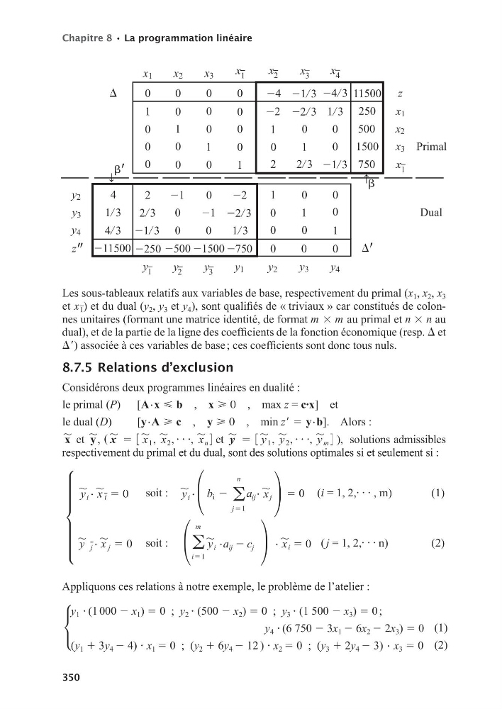
Les sous- tableaux rela tifs aux variables de base, res pec ti ve ment du primal (x 1 , x 2 , x 3
et x 1 ) et du dual (y 2 , y 3 et y 4 ),sontqua li fiésde«tri viaux»carconsti tuésdecolonnes uni taires (for mant une matrice iden tité, de for mat m 3 m au primal et n 3 n au
dual),etdelapar tiedelalignedescoef fi cientsdelafonc tionéco no mique(resp.D et
Dr)asso ciéeàcesvariablesdebase;cescoefficientssontdonctousnuls.
8.7.5 Rela tions d’exclu sion
Consi dé rons deux pro grammes linéaires en dua lité :
le primal (P) [A # x < b , x > 0 , max z = c∙x] et
le dual (D)
[y # A > c , y > 0 , min zr 5 y # b]. Alors :
x
, et y
, , ( x
, 5 3 x
,
1 , x
,
2 , c , x
,
n 4 et y
, 5 3 y
,
1 , y
,
2 , c , y
,
m 4 ), solu tions admis sibles
res pec ti ve ment du primal et du dual, sont des solu tions opti males si et seule ment si :
f
y
,
i
# x
,
i 5 0 soit : y
,
i
# £ b i 2 a
n
j51
a ij # x
,
j ≥ 5 0 (i = 1, 2, c , m)
(1)
y
, j # x
,
j 5 0 soit : £ a
m
i51
y
,
i
# a ij 2 c j ≥ # x
,
i 5 0 ( j = 1, 2, c n)
(2)
Appli quons ces rela tions à notre exemple, le problème de l’atelier :
c
y 1 ? (1 000 2 x 1 ) 5 0 ; y 2 ? (500 2 x 2 ) 5 0 ; y 3 ? (1 500 2 x 3 ) 5 0 ;
y 4 ? (6 750 2 3x 1 2 6x 2 2 2x 3 ) 5 0 (1)
(y 1 1 3y 4 2 4) ? x 1 5 0 ; (y 2 1 6y 4 2 12 ) ? x 2 5 0 ; (y 3 1 2y 4 2 3) # x 3 5 0 (2)
350
x 1
x 1
x 1
z
x 2
x 2
x 3
x 3 Primal
Dual
x 1
x 2
x 3
x 4
y 2
y 3
y 4
y 2
y 1
y 4
y 1
y 3
y 2
y 3
z
1/ 3
4/ 3
1/ 3
1/ 3
2/ 3
4/ 3
2/ 3
1/ 3
1/ 3
4
2
2
2
2
4
1
1500
1500
750
750
500
500
250
250
11500
11500
1
1/ 3
2/ 3
2/ 3
0
0
0
0
0
0
0
0
0
0
0
0
0
0
0
0
0
0
0
0
0
0
0
0
0
0
0
0
0
0
0
0
0
1
1
1
1
1
1
1
1
1
↑
↑
Les sous- tableaux rela tifs aux variables de base, res pec ti ve ment du primal (x 1 , x 2 , x 3
et x 1 ) et du dual (y 2 , y 3 et y 4 ),sontqua li fiésde«tri viaux»carconsti tuésdecolonnes uni taires (for mant une matrice iden tité, de for mat m 3 m au primal et n 3 n au
dual),etdelapar tiedelalignedescoef fi cientsdelafonc tionéco no mique(resp.D et
Dr)asso ciéeàcesvariablesdebase;cescoefficientssontdonctousnuls.
8.7.5 Rela tions d’exclu sion
Consi dé rons deux pro grammes linéaires en dua lité :
le primal (P) [A # x < b , x > 0 , max z = c∙x] et
le dual (D)
[y # A > c , y > 0 , min zr 5 y # b]. Alors :
x
, et y
, , ( x
, 5 3 x
,
1 , x
,
2 , c , x
,
n 4 et y
, 5 3 y
,
1 , y
,
2 , c , y
,
m 4 ), solu tions admis sibles
res pec ti ve ment du primal et du dual, sont des solu tions opti males si et seule ment si :
f
y
,
i
# x
,
i 5 0 soit : y
,
i
# £ b i 2 a
n
j51
a ij # x
,
j ≥ 5 0 (i = 1, 2, c , m)
(1)
y
, j # x
,
j 5 0 soit : £ a
m
i51
y
,
i
# a ij 2 c j ≥ # x
,
i 5 0 ( j = 1, 2, c n)
(2)
Appli quons ces rela tions à notre exemple, le problème de l’atelier :
c
y 1 ? (1 000 2 x 1 ) 5 0 ; y 2 ? (500 2 x 2 ) 5 0 ; y 3 ? (1 500 2 x 3 ) 5 0 ;
y 4 ? (6 750 2 3x 1 2 6x 2 2 2x 3 ) 5 0 (1)
(y 1 1 3y 4 2 4) ? x 1 5 0 ; (y 2 1 6y 4 2 12 ) ? x 2 5 0 ; (y 3 1 2y 4 2 3) # x 3 5 0 (2)