

72
4 Measurement of Work Function
metal
vacuum
Work
funcƟon
Tunneling electrons
Strong electric field
Valence band
Electric field = 0
Thermal
excitaƟon
Extract electrons via
strong field
Photon
excitaƟon
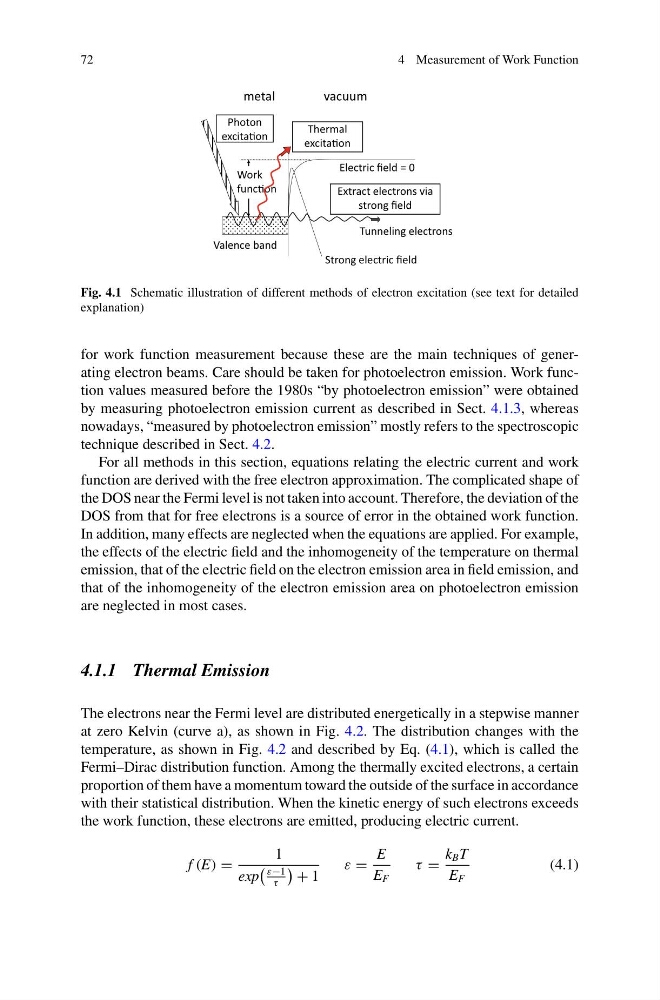
Fig. 4.1 Schematic illustration of different methods of electron excitation (see text for detailed
explanation)
for work function measurement because these are the main techniques of generating electron beams. Care should be taken for photoelectron emission. Work function values measured before the 1980s “by photoelectron emission” were obtained
by measuring photoelectron emission current as described in Sect. 4.1.3, whereas
nowadays, “measured by photoelectron emission” mostly refers to the spectroscopic
technique described in Sect. 4.2.
For all methods in this section, equations relating the electric current and work
function are derived with the free electron approximation. The complicated shape of
the DOS near the Fermi level is not taken into account. Therefore, the deviation of the
DOS from that for free electrons is a source of error in the obtained work function.
In addition, many effects are neglected when the equations are applied. For example,
the effects of the electric field and the inhomogeneity of the temperature on thermal
emission, that of the electric field on the electron emission area in field emission, and
that of the inhomogeneity of the electron emission area on photoelectron emission
are neglected in most cases.
4.1.1 Thermal Emission
The electrons near the Fermi level are distributed energetically in a stepwise manner
at zero Kelvin (curve a), as shown in Fig. 4.2. The distribution changes with the
temperature, as shown in Fig. 4.2 and described by Eq. (4.1), which is called the
Fermi–Dirac distribution function. Among the thermally excited electrons, a certain
proportion of them have a momentum toward the outside of the surface in accordance
with their statistical distribution. When the kinetic energy of such electrons exceeds
the work function, these electrons are emitted, producing electric current.
f (E) =
1
exp
ε−1
τ
+ 1
ε =
E
E F
τ =
k B T
E F
(4.1)
4 Measurement of Work Function
metal
vacuum
Work
funcƟon
Tunneling electrons
Strong electric field
Valence band
Electric field = 0
Thermal
excitaƟon
Extract electrons via
strong field
Photon
excitaƟon
Fig. 4.1 Schematic illustration of different methods of electron excitation (see text for detailed
explanation)
for work function measurement because these are the main techniques of generating electron beams. Care should be taken for photoelectron emission. Work function values measured before the 1980s “by photoelectron emission” were obtained
by measuring photoelectron emission current as described in Sect. 4.1.3, whereas
nowadays, “measured by photoelectron emission” mostly refers to the spectroscopic
technique described in Sect. 4.2.
For all methods in this section, equations relating the electric current and work
function are derived with the free electron approximation. The complicated shape of
the DOS near the Fermi level is not taken into account. Therefore, the deviation of the
DOS from that for free electrons is a source of error in the obtained work function.
In addition, many effects are neglected when the equations are applied. For example,
the effects of the electric field and the inhomogeneity of the temperature on thermal
emission, that of the electric field on the electron emission area in field emission, and
that of the inhomogeneity of the electron emission area on photoelectron emission
are neglected in most cases.
4.1.1 Thermal Emission
The electrons near the Fermi level are distributed energetically in a stepwise manner
at zero Kelvin (curve a), as shown in Fig. 4.2. The distribution changes with the
temperature, as shown in Fig. 4.2 and described by Eq. (4.1), which is called the
Fermi–Dirac distribution function. Among the thermally excited electrons, a certain
proportion of them have a momentum toward the outside of the surface in accordance
with their statistical distribution. When the kinetic energy of such electrons exceeds
the work function, these electrons are emitted, producing electric current.
f (E) =
1
exp
ε−1
τ
+ 1
ε =
E
E F
τ =
k B T
E F
(4.1)