

crystals are grown one shell after the other. For example, in the case of a zinc
blende structure, we start with the central cation surrounded by the four neighboring anions. These four anions are then bonded to twelve cations in the next
shell and so on till we reach the desired size of the nanocrystal. Then, the e’s and
t’s are assigned to the various orbitals and pairs of orbitals, respectively, thereby
generating the Hamiltonian matrix. The TB-Hamiltonian matrix thus generated is
then diagonalized to obtain the eigenvalue spectra. For small sized matrices, direct
diagonalization works well, but it becomes progressively more time consuming
and eventually almost impossible to diagonalize the Hamiltonian matrix as the size
of the nanocrystal grows. Therefore, for larger nanocrystals we revert to more effcient techniques such as the Lanczos algorithm [65]. Calculations for different
sized nanocrystal provide us with the dependence of the band gap on size.
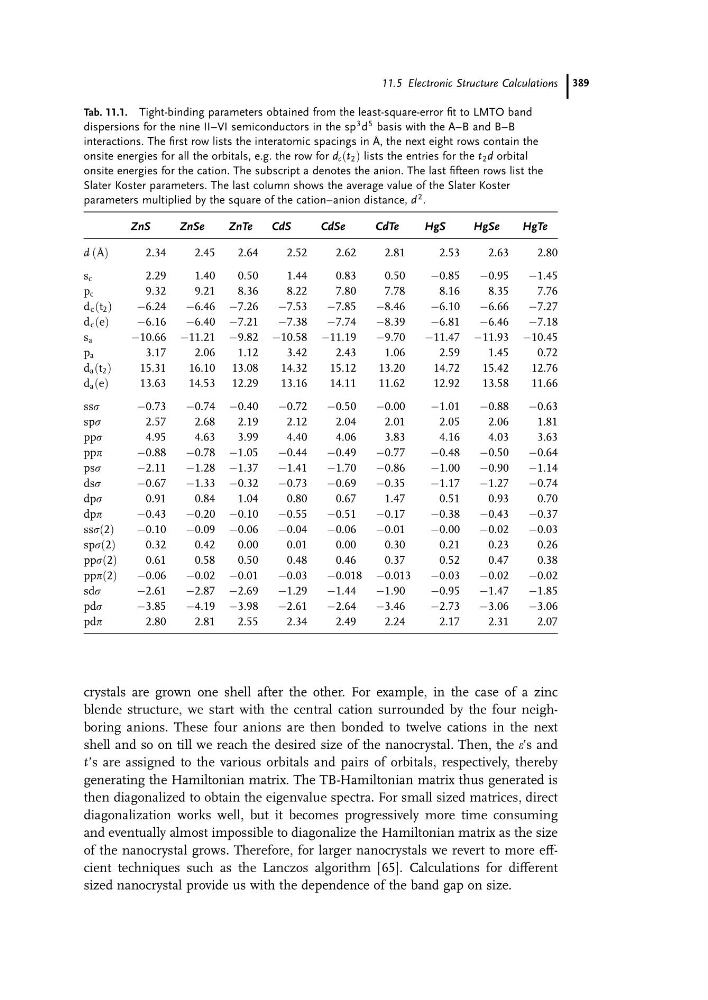
Tab. 11.1. Tight-binding parameters obtained from the least-square-error fit to LMTO band
dispersions for the nine II–VI semiconductors in the sp
3 d
5 basis with the A–B and B–B
interactions. The first row lists the interatomic spacings in A ˚ , the next eight rows contain the
onsite energies for all the orbitals, e.g. the row for d c ðt 2 Þ lists the entries for the t 2 d orbital
onsite energies for the cation. The subscript a denotes the anion. The last fifteen rows list the
Slater Koster parameters. The last column shows the average value of the Slater Koster
parameters multiplied by the square of the cation–anion distance, d
2 .
ZnS
ZnSe
ZnTe
CdS
CdSe
CdTe
HgS
HgSe
HgTe
d (A ˚ )
2.34
2.45
2.64
2.52
2.62
2.81
2.53
2.63
2.80
s c
2.29
1.40
0.50
1.44
0.83
0.50
À0.85
À0.95
À1.45
p c
9.32
9.21
8.36
8.22
7.80
7.78
8.16
8.35
7.76
d c ðt 2 Þ
À6.24
À6.46 À7.26
À7.53
À7.85
À8.46
À6.10
À6.66
À7.27
d c ðeÞ
À6.16
À6.40 À7.21
À7.38
À7.74
À8.39
À6.81
À6.46
À7.18
s a
À10.66 À11.21 À9.82 À10.58 À11.19
À9.70
À11.47 À11.93 À10.45
p a
3.17
2.06
1.12
3.42
2.43
1.06
2.59
1.45
0.72
d a ðt 2 Þ
15.31
16.10 13.08
14.32
15.12
13.20
14.72
15.42
12.76
d a ðeÞ
13.63
14.53 12.29
13.16
14.11
11.62
12.92
13.58
11.66
sss
À0.73
À0.74 À0.40
À0.72
À0.50
À0.00
À1.01
À0.88
À0.63
sps
2.57
2.68
2.19
2.12
2.04
2.01
2.05
2.06
1.81
pps
4.95
4.63
3.99
4.40
4.06
3.83
4.16
4.03
3.63
ppp
À0.88
À0.78 À1.05
À0.44
À0.49
À0.77
À0.48
À0.50
À0.64
pss
À2.11
À1.28 À1.37
À1.41
À1.70
À0.86
À1.00
À0.90
À1.14
dss
À0.67
À1.33 À0.32
À0.73
À0.69
À0.35
À1.17
À1.27
À0.74
dps
0.91
0.84
1.04
0.80
0.67
1.47
0.51
0.93
0.70
dpp
À0.43
À0.20 À0.10
À0.55
À0.51
À0.17
À0.38
À0.43
À0.37
sssð2Þ
À0.10
À0.09 À0.06
À0.04
À0.06
À0.01
À0.00
À0.02
À0.03
spsð2Þ
0.32
0.42
0.00
0.01
0.00
0.30
0.21
0.23
0.26
ppsð2Þ
0.61
0.58
0.50
0.48
0.46
0.37
0.52
0.47
0.38
pppð2Þ
À0.06
À0.02 À0.01
À0.03
À0.018 À0.013
À0.03
À0.02
À0.02
sds
À2.61
À2.87 À2.69
À1.29
À1.44
À1.90
À0.95
À1.47
À1.85
pds
À3.85
À4.19 À3.98
À2.61
À2.64
À3.46
À2.73
À3.06
À3.06
pdp
2.80
2.81
2.55
2.34
2.49
2.24
2.17
2.31
2.07
11.5 Electronic Structure Calculations 389
blende structure, we start with the central cation surrounded by the four neighboring anions. These four anions are then bonded to twelve cations in the next
shell and so on till we reach the desired size of the nanocrystal. Then, the e’s and
t’s are assigned to the various orbitals and pairs of orbitals, respectively, thereby
generating the Hamiltonian matrix. The TB-Hamiltonian matrix thus generated is
then diagonalized to obtain the eigenvalue spectra. For small sized matrices, direct
diagonalization works well, but it becomes progressively more time consuming
and eventually almost impossible to diagonalize the Hamiltonian matrix as the size
of the nanocrystal grows. Therefore, for larger nanocrystals we revert to more effcient techniques such as the Lanczos algorithm [65]. Calculations for different
sized nanocrystal provide us with the dependence of the band gap on size.
Tab. 11.1. Tight-binding parameters obtained from the least-square-error fit to LMTO band
dispersions for the nine II–VI semiconductors in the sp
3 d
5 basis with the A–B and B–B
interactions. The first row lists the interatomic spacings in A ˚ , the next eight rows contain the
onsite energies for all the orbitals, e.g. the row for d c ðt 2 Þ lists the entries for the t 2 d orbital
onsite energies for the cation. The subscript a denotes the anion. The last fifteen rows list the
Slater Koster parameters. The last column shows the average value of the Slater Koster
parameters multiplied by the square of the cation–anion distance, d
2 .
ZnS
ZnSe
ZnTe
CdS
CdSe
CdTe
HgS
HgSe
HgTe
d (A ˚ )
2.34
2.45
2.64
2.52
2.62
2.81
2.53
2.63
2.80
s c
2.29
1.40
0.50
1.44
0.83
0.50
À0.85
À0.95
À1.45
p c
9.32
9.21
8.36
8.22
7.80
7.78
8.16
8.35
7.76
d c ðt 2 Þ
À6.24
À6.46 À7.26
À7.53
À7.85
À8.46
À6.10
À6.66
À7.27
d c ðeÞ
À6.16
À6.40 À7.21
À7.38
À7.74
À8.39
À6.81
À6.46
À7.18
s a
À10.66 À11.21 À9.82 À10.58 À11.19
À9.70
À11.47 À11.93 À10.45
p a
3.17
2.06
1.12
3.42
2.43
1.06
2.59
1.45
0.72
d a ðt 2 Þ
15.31
16.10 13.08
14.32
15.12
13.20
14.72
15.42
12.76
d a ðeÞ
13.63
14.53 12.29
13.16
14.11
11.62
12.92
13.58
11.66
sss
À0.73
À0.74 À0.40
À0.72
À0.50
À0.00
À1.01
À0.88
À0.63
sps
2.57
2.68
2.19
2.12
2.04
2.01
2.05
2.06
1.81
pps
4.95
4.63
3.99
4.40
4.06
3.83
4.16
4.03
3.63
ppp
À0.88
À0.78 À1.05
À0.44
À0.49
À0.77
À0.48
À0.50
À0.64
pss
À2.11
À1.28 À1.37
À1.41
À1.70
À0.86
À1.00
À0.90
À1.14
dss
À0.67
À1.33 À0.32
À0.73
À0.69
À0.35
À1.17
À1.27
À0.74
dps
0.91
0.84
1.04
0.80
0.67
1.47
0.51
0.93
0.70
dpp
À0.43
À0.20 À0.10
À0.55
À0.51
À0.17
À0.38
À0.43
À0.37
sssð2Þ
À0.10
À0.09 À0.06
À0.04
À0.06
À0.01
À0.00
À0.02
À0.03
spsð2Þ
0.32
0.42
0.00
0.01
0.00
0.30
0.21
0.23
0.26
ppsð2Þ
0.61
0.58
0.50
0.48
0.46
0.37
0.52
0.47
0.38
pppð2Þ
À0.06
À0.02 À0.01
À0.03
À0.018 À0.013
À0.03
À0.02
À0.02
sds
À2.61
À2.87 À2.69
À1.29
À1.44
À1.90
À0.95
À1.47
À1.85
pds
À3.85
À4.19 À3.98
À2.61
À2.64
À3.46
À2.73
À3.06
À3.06
pdp
2.80
2.81
2.55
2.34
2.49
2.24
2.17
2.31
2.07
11.5 Electronic Structure Calculations 389