

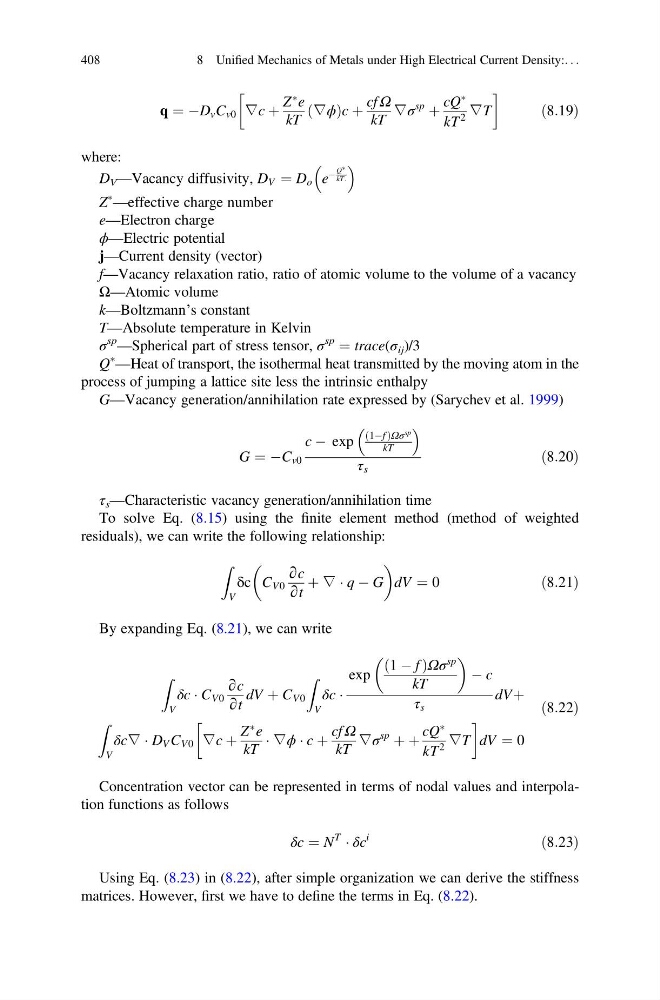
q ¼ ÀD v C v0 ∇c þ
Z
à e
kT
∇ϕ
ð
Þc þ
cf Ω
kT
∇σ
sp
þ
cQ
Ã
kT
2
∇T
!
ð8:19Þ
where:
D V —Vacancy diffusivity, D V ¼ D o e
À
Q Ã
kT:
Z
Ã
—effective charge number
e—Electron charge
ϕ—Electric potential
j—Current density (vector)
f—Vacancy relaxation ratio, ratio of atomic volume to the volume of a vacancy
Ω—Atomic volume
k—Boltzmann’s constant
T—Absolute temperature in Kelvin
σ
sp
—Spherical part of stress tensor, σ
sp
¼ trace(σ ij )/3
Q
Ã
—Heat of transport, the isothermal heat transmitted by the moving atom in the
process of jumping a lattice site less the intrinsic enthalpy
G—Vacancy generation/annihilation rate expressed by (Sarychev et al. 1999)
G ¼ ÀC v0
c À exp
1Àf
ð
ÞΩσ
sp
kT
τ s
ð8:20Þ
τ s —Characteristic vacancy generation/annihilation time
To solve Eq. (8.15) using the finite element method (method of weighted
residuals), we can write the following relationship:
Z
V
δc C V0
∂c
∂t
þ ∇ Á q À G
dV ¼ 0
ð8:21Þ
By expanding Eq. (8.21), we can write
Z
V
δc Á C V0
∂c
∂t
dV þ C V0
Z
V
δc Á
exp
1 À f
ð
ÞΩσ
sp
kT
À c
τ s
dVþ
Z
V
δc∇ Á D V C V0 ∇c þ
Z
à e
kT
Á ∇ϕ Á c þ
cf Ω
kT
∇σ
sp
þ þ
cQ
Ã
kT
2
∇T
!
dV ¼ 0
ð8:22Þ
Concentration vector can be represented in terms of nodal values and interpolation functions as follows
δc ¼ N
T
Á δc
i
ð8:23Þ
Using Eq. (8.23) in (8.22), after simple organization we can derive the stiffness
matrices. However, first we have to define the terms in Eq. (8.22).
408
8 Unified Mechanics of Metals under High Electrical Current Density:. . .
Z
à e
kT
∇ϕ
ð
Þc þ
cf Ω
kT
∇σ
sp
þ
cQ
Ã
kT
2
∇T
!
ð8:19Þ
where:
D V —Vacancy diffusivity, D V ¼ D o e
À
Q Ã
kT:
Z
Ã
—effective charge number
e—Electron charge
ϕ—Electric potential
j—Current density (vector)
f—Vacancy relaxation ratio, ratio of atomic volume to the volume of a vacancy
Ω—Atomic volume
k—Boltzmann’s constant
T—Absolute temperature in Kelvin
σ
sp
—Spherical part of stress tensor, σ
sp
¼ trace(σ ij )/3
Q
Ã
—Heat of transport, the isothermal heat transmitted by the moving atom in the
process of jumping a lattice site less the intrinsic enthalpy
G—Vacancy generation/annihilation rate expressed by (Sarychev et al. 1999)
G ¼ ÀC v0
c À exp
1Àf
ð
ÞΩσ
sp
kT
τ s
ð8:20Þ
τ s —Characteristic vacancy generation/annihilation time
To solve Eq. (8.15) using the finite element method (method of weighted
residuals), we can write the following relationship:
Z
V
δc C V0
∂c
∂t
þ ∇ Á q À G
dV ¼ 0
ð8:21Þ
By expanding Eq. (8.21), we can write
Z
V
δc Á C V0
∂c
∂t
dV þ C V0
Z
V
δc Á
exp
1 À f
ð
ÞΩσ
sp
kT
À c
τ s
dVþ
Z
V
δc∇ Á D V C V0 ∇c þ
Z
à e
kT
Á ∇ϕ Á c þ
cf Ω
kT
∇σ
sp
þ þ
cQ
Ã
kT
2
∇T
!
dV ¼ 0
ð8:22Þ
Concentration vector can be represented in terms of nodal values and interpolation functions as follows
δc ¼ N
T
Á δc
i
ð8:23Þ
Using Eq. (8.23) in (8.22), after simple organization we can derive the stiffness
matrices. However, first we have to define the terms in Eq. (8.22).
408
8 Unified Mechanics of Metals under High Electrical Current Density:. . .