

M
ep
nþ1 ¼
κI I þ 2μδ nþ1
b
‘ À
1
3
I I
À 2μθ nþ1 b n nþ1 b n nþ1
À
2μ
b
K
b n nþ1 b v nþ1
À
2μ
b
K
b n nþ1 b v nþ1
2μδ nþ1
b
‘ À 2μθ nþ1 v nþ1 b v nþ1
2
6
6
4
3
7
7
5
ð5:221Þ
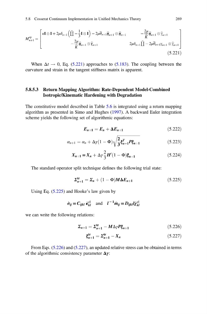
When Δt ! 0, Eq. (5.221) approaches to (5.183). The coupling between the
curvature and strain in the tangent stiffness matrix is apparent.
5.8.5.3 Return Mapping Algorithm: Rate-Dependent Model-Combined
Isotropic/Kinematic Hardening with Degradation
The constitutive model described in Table 5.6 is integrated using a return mapping
algorithm as presented in Simo and Hughes (1997). A backward Euler integration
scheme yields the following set of algorithmic equations:
Ε nþ1 ¼ Ε n þ ΔΕ nþ1
ð5:222Þ
α nþ1 ¼ α n þ Δγ 1 À Φ
ð
Þ
ffiffiffiffiffiffiffiffiffiffiffiffiffiffiffiffiffiffiffiffiffiffiffi
2
3
ξ
T
nþ1 Pξ nþ1
r
ð5:223Þ
X nþ1 = X n þ Δγ
2
3
H
0 1 À Φ
ð
Þξ nþ1
ð5:224Þ
The standard operator split technique defines the following trial state:
Σ
tr
nþ1 ¼ Σ n þ 1 À Φ
ð
ÞMΔΕ nþ1
ð5:225Þ
Using Eq. (5.225) and Hooke’s law given by
_
σ ij = C ijkl _
e
el
kl
and l
2 1
_
m ij = D ijkl l _
χ
el
kl
we can write the following relations:
Σ nþ1 ¼ Σ
tr
nþ1 À MΔγPξ nþ1
ð5:226Þ
ξ
tr
nþ1 ¼ Σ
tr
nþ1 À X n
ð5:227Þ
From Eqs. (5.226) and (5.227), an updated relative stress can be obtained in terms
of the algorithmic consistency parameter Δγ:
5.8 Cosserat Continuum Implementation in Unified Mechanics Theory
269
ep
nþ1 ¼
κI I þ 2μδ nþ1
b
‘ À
1
3
I I
À 2μθ nþ1 b n nþ1 b n nþ1
À
2μ
b
K
b n nþ1 b v nþ1
À
2μ
b
K
b n nþ1 b v nþ1
2μδ nþ1
b
‘ À 2μθ nþ1 v nþ1 b v nþ1
2
6
6
4
3
7
7
5
ð5:221Þ
When Δt ! 0, Eq. (5.221) approaches to (5.183). The coupling between the
curvature and strain in the tangent stiffness matrix is apparent.
5.8.5.3 Return Mapping Algorithm: Rate-Dependent Model-Combined
Isotropic/Kinematic Hardening with Degradation
The constitutive model described in Table 5.6 is integrated using a return mapping
algorithm as presented in Simo and Hughes (1997). A backward Euler integration
scheme yields the following set of algorithmic equations:
Ε nþ1 ¼ Ε n þ ΔΕ nþ1
ð5:222Þ
α nþ1 ¼ α n þ Δγ 1 À Φ
ð
Þ
ffiffiffiffiffiffiffiffiffiffiffiffiffiffiffiffiffiffiffiffiffiffiffi
2
3
ξ
T
nþ1 Pξ nþ1
r
ð5:223Þ
X nþ1 = X n þ Δγ
2
3
H
0 1 À Φ
ð
Þξ nþ1
ð5:224Þ
The standard operator split technique defines the following trial state:
Σ
tr
nþ1 ¼ Σ n þ 1 À Φ
ð
ÞMΔΕ nþ1
ð5:225Þ
Using Eq. (5.225) and Hooke’s law given by
_
σ ij = C ijkl _
e
el
kl
and l
2 1
_
m ij = D ijkl l _
χ
el
kl
we can write the following relations:
Σ nþ1 ¼ Σ
tr
nþ1 À MΔγPξ nþ1
ð5:226Þ
ξ
tr
nþ1 ¼ Σ
tr
nþ1 À X n
ð5:227Þ
From Eqs. (5.226) and (5.227), an updated relative stress can be obtained in terms
of the algorithmic consistency parameter Δγ:
5.8 Cosserat Continuum Implementation in Unified Mechanics Theory
269