

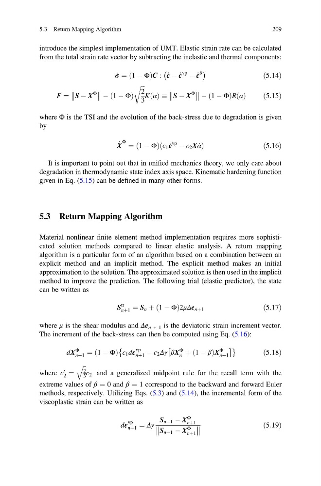
introduce the simplest implementation of UMT. Elastic strain rate can be calculated
from the total strain rate vector by subtracting the inelastic and thermal components:
_
σ ¼ 1 À Φ
ð
ÞC : _
ε À _
ε
vp
À _
ε
θ
À
Á
ð5:14Þ
F ¼ S À X
Φ
À 1 À Φ
ð
Þ
ffiffi ffi
2
3
r
K α
ð Þ S À X
Φ
À 1 À Φ
ð
ÞR α
ð Þ
ð5:15Þ
where Φ is the TSI and the evolution of the back-stress due to degradation is given
by
_
X
Φ ¼ 1 À Φ
ð
Þ c 1 _
ε
vp
À c 2 X _
α
ð
Þ
ð 5:16Þ
It is important to point out that in unified mechanics theory, we only care about
degradation in thermodynamic state index axis space. Kinematic hardening function
given in Eq. (5.15) can be defined in many other forms.
5.3 Return Mapping Algorithm
Material nonlinear finite element method implementation requires more sophisticated solution methods compared to linear elastic analysis. A return mapping
algorithm is a particular form of an algorithm based on a combination between an
explicit method and an implicit method. The explicit method makes an initial
approximation to the solution. The approximated solution is then used in the implicit
method to improve the prediction. The following trial (elastic predictor), the state
can be written as
S
tr
nþ1 ¼ S n þ 1 À Φ
ð
Þ2μΔe nþ1
ð5:17Þ
where μ is the shear modulus and Δe n + 1 is the deviatoric strain increment vector.
The increment of the back-stress can then be computed using Eq. (5.16):
dX
Φ
nþ1 ¼ 1 À Φ
ð
Þ c 1 dε
vp
nþ1 À c 2 Δγ βX
Φ
n þ 1 À β
ð
ÞX
Φ
nþ1
Â
Ã
È
É
ð5:18Þ
where c
0
2 ¼
ffiffi
2
3
q
c 2 and a generalized midpoint rule for the recall term with the
extreme values of β ¼ 0 and β ¼ 1 correspond to the backward and forward Euler
methods, respectively. Utilizing Eqs. (5.3) and (5.14), the incremental form of the
viscoplastic strain can be written as
dε
vp
nþ1 ¼ Δγ
S nþ1 À X
Φ
nþ1
S nþ1 À X
Φ
nþ1
ð5:19Þ
5.3 Return Mapping Algorithm
209
from the total strain rate vector by subtracting the inelastic and thermal components:
_
σ ¼ 1 À Φ
ð
ÞC : _
ε À _
ε
vp
À _
ε
θ
À
Á
ð5:14Þ
F ¼ S À X
Φ
À 1 À Φ
ð
Þ
ffiffi ffi
2
3
r
K α
ð Þ S À X
Φ
À 1 À Φ
ð
ÞR α
ð Þ
ð5:15Þ
where Φ is the TSI and the evolution of the back-stress due to degradation is given
by
_
X
Φ ¼ 1 À Φ
ð
Þ c 1 _
ε
vp
À c 2 X _
α
ð
Þ
ð 5:16Þ
It is important to point out that in unified mechanics theory, we only care about
degradation in thermodynamic state index axis space. Kinematic hardening function
given in Eq. (5.15) can be defined in many other forms.
5.3 Return Mapping Algorithm
Material nonlinear finite element method implementation requires more sophisticated solution methods compared to linear elastic analysis. A return mapping
algorithm is a particular form of an algorithm based on a combination between an
explicit method and an implicit method. The explicit method makes an initial
approximation to the solution. The approximated solution is then used in the implicit
method to improve the prediction. The following trial (elastic predictor), the state
can be written as
S
tr
nþ1 ¼ S n þ 1 À Φ
ð
Þ2μΔe nþ1
ð5:17Þ
where μ is the shear modulus and Δe n + 1 is the deviatoric strain increment vector.
The increment of the back-stress can then be computed using Eq. (5.16):
dX
Φ
nþ1 ¼ 1 À Φ
ð
Þ c 1 dε
vp
nþ1 À c 2 Δγ βX
Φ
n þ 1 À β
ð
ÞX
Φ
nþ1
Â
Ã
È
É
ð5:18Þ
where c
0
2 ¼
ffiffi
2
3
q
c 2 and a generalized midpoint rule for the recall term with the
extreme values of β ¼ 0 and β ¼ 1 correspond to the backward and forward Euler
methods, respectively. Utilizing Eqs. (5.3) and (5.14), the incremental form of the
viscoplastic strain can be written as
dε
vp
nþ1 ¼ Δγ
S nþ1 À X
Φ
nþ1
S nþ1 À X
Φ
nþ1
ð5:19Þ
5.3 Return Mapping Algorithm
209