

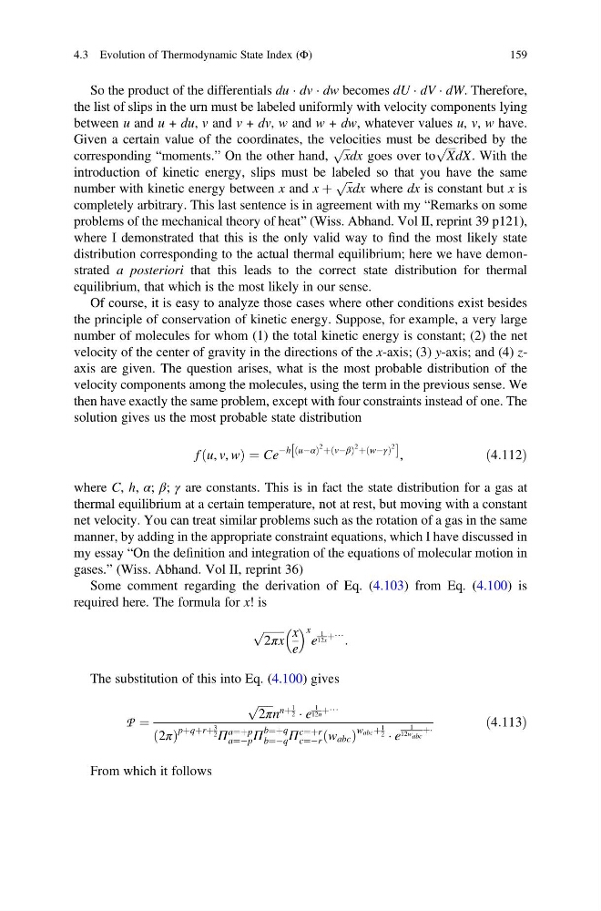
So the product of the differentials du Á dv Á dw becomes dU Á dV Á dW. Therefore,
the list of slips in the urn must be labeled uniformly with velocity components lying
between u and u + du, v and v + dv, w and w + dw, whatever values u, v, w have.
Given a certain value of the coordinates, the velocities must be described by the
corresponding “moments.” On the other hand,
ffiffi ffi
x
p
dx goes over to
ffiffiffi ffi
X
p
dX. With the
introduction of kinetic energy, slips must be labeled so that you have the same
number with kinetic energy between x and x þ
ffiffi ffi
x
p
dx where dx is constant but x is
completely arbitrary. This last sentence is in agreement with my “Remarks on some
problems of the mechanical theory of heat” (Wiss. Abhand. Vol II, reprint 39 p121),
where I demonstrated that this is the only valid way to find the most likely state
distribution corresponding to the actual thermal equilibrium; here we have demonstrated a posteriori that this leads to the correct state distribution for thermal
equilibrium, that which is the most likely in our sense.
Of course, it is easy to analyze those cases where other conditions exist besides
the principle of conservation of kinetic energy. Suppose, for example, a very large
number of molecules for whom (1) the total kinetic energy is constant; (2) the net
velocity of the center of gravity in the directions of the x-axis; (3) y-axis; and (4) zaxis are given. The question arises, what is the most probable distribution of the
velocity components among the molecules, using the term in the previous sense. We
then have exactly the same problem, except with four constraints instead of one. The
solution gives us the most probable state distribution
f u, v, w
ð
Þ¼Ce
Àh uÀα
ð
Þ
2 þ vÀβ
ð
Þ
2 þ wÀγ
ð
Þ
2
½
,
ð4:112Þ
where C, h, α; β; γ are constants. This is in fact the state distribution for a gas at
thermal equilibrium at a certain temperature, not at rest, but moving with a constant
net velocity. You can treat similar problems such as the rotation of a gas in the same
manner, by adding in the appropriate constraint equations, which I have discussed in
my essay “On the definition and integration of the equations of molecular motion in
gases.” (Wiss. Abhand. Vol II, reprint 36)
Some comment regarding the derivation of Eq. (4.103) from Eq. (4.100) is
required here. The formula for x! is
ffiffiffiffiffiffiffi ffi
2πx
p
x
e
x
e
1
12x þ⋯
:
The substitution of this into Eq. (4.100) gives
P ¼
ffiffiffiffiffi
2π
p
n
nþ
1
2 Á e
1
12n þ⋯
2π
ð Þ
pþqþrþ
3
2 Π
a¼þp
a¼Àp Π
b¼þq
b¼Àq Π
c¼þr
c¼Àr w abc
ð
Þ
w abc þ
1
2 Á e
1
12w abc
þÁ
ð4:113Þ
From which it follows
4.3 Evolution of Thermodynamic State Index (Φ)
159
the list of slips in the urn must be labeled uniformly with velocity components lying
between u and u + du, v and v + dv, w and w + dw, whatever values u, v, w have.
Given a certain value of the coordinates, the velocities must be described by the
corresponding “moments.” On the other hand,
ffiffi ffi
x
p
dx goes over to
ffiffiffi ffi
X
p
dX. With the
introduction of kinetic energy, slips must be labeled so that you have the same
number with kinetic energy between x and x þ
ffiffi ffi
x
p
dx where dx is constant but x is
completely arbitrary. This last sentence is in agreement with my “Remarks on some
problems of the mechanical theory of heat” (Wiss. Abhand. Vol II, reprint 39 p121),
where I demonstrated that this is the only valid way to find the most likely state
distribution corresponding to the actual thermal equilibrium; here we have demonstrated a posteriori that this leads to the correct state distribution for thermal
equilibrium, that which is the most likely in our sense.
Of course, it is easy to analyze those cases where other conditions exist besides
the principle of conservation of kinetic energy. Suppose, for example, a very large
number of molecules for whom (1) the total kinetic energy is constant; (2) the net
velocity of the center of gravity in the directions of the x-axis; (3) y-axis; and (4) zaxis are given. The question arises, what is the most probable distribution of the
velocity components among the molecules, using the term in the previous sense. We
then have exactly the same problem, except with four constraints instead of one. The
solution gives us the most probable state distribution
f u, v, w
ð
Þ¼Ce
Àh uÀα
ð
Þ
2 þ vÀβ
ð
Þ
2 þ wÀγ
ð
Þ
2
½
,
ð4:112Þ
where C, h, α; β; γ are constants. This is in fact the state distribution for a gas at
thermal equilibrium at a certain temperature, not at rest, but moving with a constant
net velocity. You can treat similar problems such as the rotation of a gas in the same
manner, by adding in the appropriate constraint equations, which I have discussed in
my essay “On the definition and integration of the equations of molecular motion in
gases.” (Wiss. Abhand. Vol II, reprint 36)
Some comment regarding the derivation of Eq. (4.103) from Eq. (4.100) is
required here. The formula for x! is
ffiffiffiffiffiffiffi ffi
2πx
p
x
e
x
e
1
12x þ⋯
:
The substitution of this into Eq. (4.100) gives
P ¼
ffiffiffiffiffi
2π
p
n
nþ
1
2 Á e
1
12n þ⋯
2π
ð Þ
pþqþrþ
3
2 Π
a¼þp
a¼Àp Π
b¼þq
b¼Àq Π
c¼þr
c¼Àr w abc
ð
Þ
w abc þ
1
2 Á e
1
12w abc
þÁ
ð4:113Þ
From which it follows
4.3 Evolution of Thermodynamic State Index (Φ)
159