

2.5 Single-Mode Fibers
67
transverse offset, variable aperture in the far field, knife-edge, and mask methods.
The main consideration of all these methods is how to approximate the optical power
distribution.
A standard technique to find the MFD is to measure the far-field intensity
distribution E
2 (r) and then calculate the MFD using the Petermann II equation [28]
MFD = 2w 0 = 2
2
∞
0 E
2
(r )r
3 dr
∞
0 E 2 (r )rdr
1/2
(2.32)
where the parameter 2w 0 (with w 0 being called the spot size or the mode field radius)
is the full width of the far-field distribution. For calculation simplicity the exact field
distribution can be fitted to a Gaussian function [22]
E(r ) = E 0 ex p
−r
2
/w
2
0
(2.33)
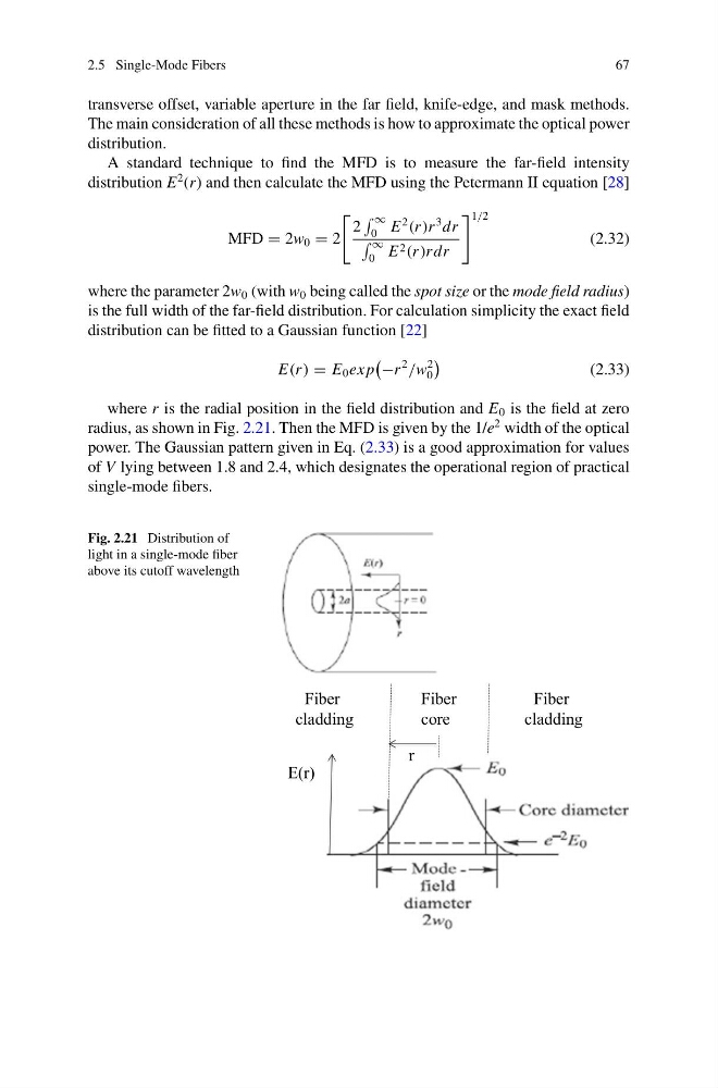
where r is the radial position in the field distribution and E 0 is the field at zero
radius, as shown in Fig. 2.21. Then the MFD is given by the 1/e
2 width of the optical
power. The Gaussian pattern given in Eq. (2.33) is a good approximation for values
of V lying between 1.8 and 2.4, which designates the operational region of practical
single-mode fibers.
Fig. 2.21 Distribution of
light in a single-mode fiber
above its cutoff wavelength
Fiber
core
Fiber
cladding
Fiber
cladding
r
E(r)
67
transverse offset, variable aperture in the far field, knife-edge, and mask methods.
The main consideration of all these methods is how to approximate the optical power
distribution.
A standard technique to find the MFD is to measure the far-field intensity
distribution E
2 (r) and then calculate the MFD using the Petermann II equation [28]
MFD = 2w 0 = 2
2
∞
0 E
2
(r )r
3 dr
∞
0 E 2 (r )rdr
1/2
(2.32)
where the parameter 2w 0 (with w 0 being called the spot size or the mode field radius)
is the full width of the far-field distribution. For calculation simplicity the exact field
distribution can be fitted to a Gaussian function [22]
E(r ) = E 0 ex p
−r
2
/w
2
0
(2.33)
where r is the radial position in the field distribution and E 0 is the field at zero
radius, as shown in Fig. 2.21. Then the MFD is given by the 1/e
2 width of the optical
power. The Gaussian pattern given in Eq. (2.33) is a good approximation for values
of V lying between 1.8 and 2.4, which designates the operational region of practical
single-mode fibers.
Fig. 2.21 Distribution of
light in a single-mode fiber
above its cutoff wavelength
Fiber
core
Fiber
cladding
Fiber
cladding
r
E(r)