

280
7 Optical Receiver Operation
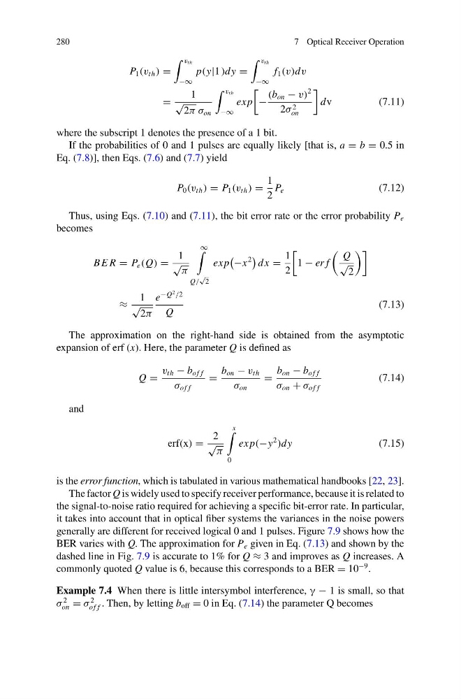
P 1 (v th ) =
v th
−∞
p(y|1 )dy =
v th
−∞
f 1 (v)dv
=
1
√
2π σ on
v th
−∞
ex p
−
(b on − v)
2
2σ 2
on
dv
(7.11)
where the subscript 1 denotes the presence of a 1 bit.
If the probabilities of 0 and 1 pulses are equally likely [that is, a = b = 0.5 in
Eq. (7.8)], then Eqs. (7.6) and (7.7) yield
P 0 (v th ) = P 1 (v th ) =
1
2
P e
(7.12)
Thus, using Eqs. (7.10) and (7.11), the bit error rate or the error probability P e
becomes
B E R = P e (Q) =
1
√
π
∞
Q/
√
2
ex p
−x
2
dx =
1
2
1 − er f
Q
√
2
≈
1
√
2π
e
−Q
2 /2
Q
(7.13)
The approximation on the right-hand side is obtained from the asymptotic
expansion of erf (x). Here, the parameter Q is defined as
Q =
v th − b of f
σ of f
=
b on − v th
σ on
=
b on − b of f
σ on + σ of f
(7.14)
and
erf(x) =
2
√
π
x
0
ex p(−y
2
)dy
(7.15)
is the error function, which is tabulated in various mathematical handbooks [22, 23].
The factor Q is widely used to specify receiver performance, because it is related to
the signal-to-noise ratio required for achieving a specific bit-error rate. In particular,
it takes into account that in optical fiber systems the variances in the noise powers
generally are different for received logical 0 and 1 pulses. Figure 7.9 shows how the
BER varies with Q. The approximation for P e given in Eq. (7.13) and shown by the
dashed line in Fig. 7.9 is accurate to 1% for Q ≈ 3 and improves as Q increases. A
commonly quoted Q value is 6, because this corresponds to a BER = 10
−9 .
Example 7.4 When there is little intersymbol interference, γ − 1 is small, so that
σ
2
on = σ
2
of f . Then, by letting b off = 0 in Eq. (7.14) the parameter Q becomes
7 Optical Receiver Operation
P 1 (v th ) =
v th
−∞
p(y|1 )dy =
v th
−∞
f 1 (v)dv
=
1
√
2π σ on
v th
−∞
ex p
−
(b on − v)
2
2σ 2
on
dv
(7.11)
where the subscript 1 denotes the presence of a 1 bit.
If the probabilities of 0 and 1 pulses are equally likely [that is, a = b = 0.5 in
Eq. (7.8)], then Eqs. (7.6) and (7.7) yield
P 0 (v th ) = P 1 (v th ) =
1
2
P e
(7.12)
Thus, using Eqs. (7.10) and (7.11), the bit error rate or the error probability P e
becomes
B E R = P e (Q) =
1
√
π
∞
Q/
√
2
ex p
−x
2
dx =
1
2
1 − er f
Q
√
2
≈
1
√
2π
e
−Q
2 /2
Q
(7.13)
The approximation on the right-hand side is obtained from the asymptotic
expansion of erf (x). Here, the parameter Q is defined as
Q =
v th − b of f
σ of f
=
b on − v th
σ on
=
b on − b of f
σ on + σ of f
(7.14)
and
erf(x) =
2
√
π
x
0
ex p(−y
2
)dy
(7.15)
is the error function, which is tabulated in various mathematical handbooks [22, 23].
The factor Q is widely used to specify receiver performance, because it is related to
the signal-to-noise ratio required for achieving a specific bit-error rate. In particular,
it takes into account that in optical fiber systems the variances in the noise powers
generally are different for received logical 0 and 1 pulses. Figure 7.9 shows how the
BER varies with Q. The approximation for P e given in Eq. (7.13) and shown by the
dashed line in Fig. 7.9 is accurate to 1% for Q ≈ 3 and improves as Q increases. A
commonly quoted Q value is 6, because this corresponds to a BER = 10
−9 .
Example 7.4 When there is little intersymbol interference, γ − 1 is small, so that
σ
2
on = σ
2
of f . Then, by letting b off = 0 in Eq. (7.14) the parameter Q becomes