

7.2 Performance Characteristics of Digital Receivers
279
f (s)ds =
1
√
2π σ
e
−(s−m)
2 /2σ
2 ds
(7.9)
where f (s) is the probability density function, σ
2 is the noise variance, and its square
root σ is the standard deviation, which is a measure of the width of the probability
distribution. By examining Eq. (7.9) it is observed that the quantity 2
√
2 σ measures
the full width of the probability distribution at the point where the amplitude is 1/e
of the maximum.
The probability density function now can be used to determine the probability of
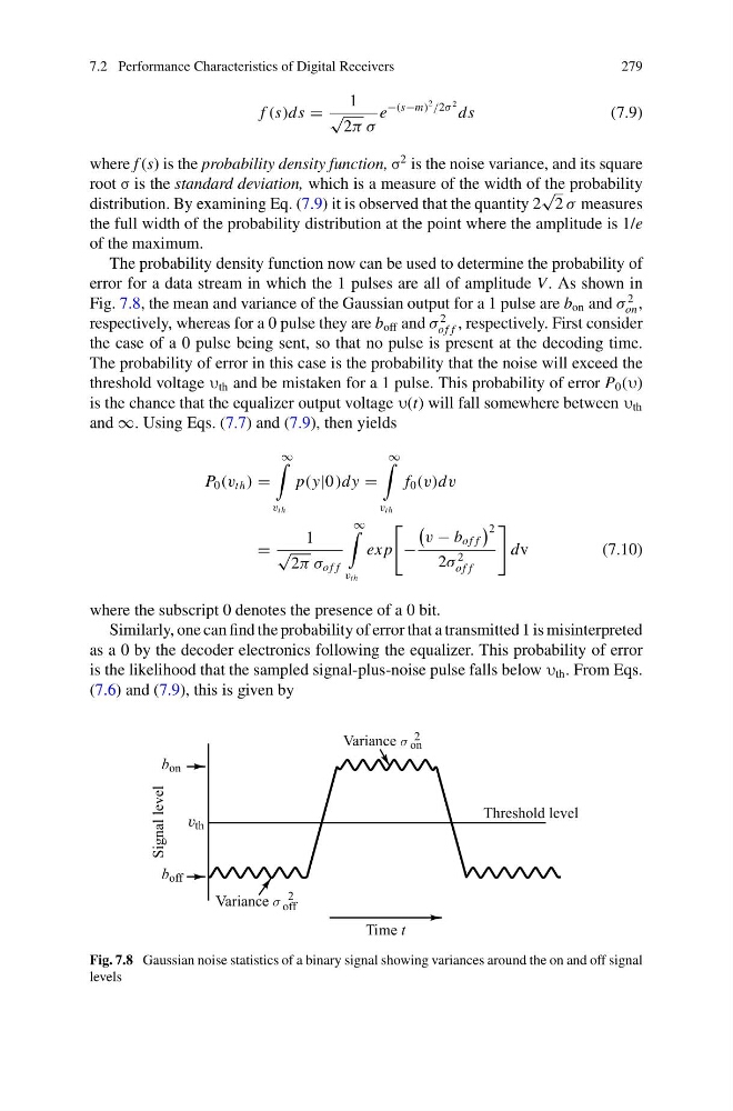
error for a data stream in which the 1 pulses are all of amplitude V. As shown in
Fig. 7.8, the mean and variance of the Gaussian output for a 1 pulse are b on and σ
2
on ,
respectively, whereas for a 0 pulse they are b off and σ
2
of f , respectively. First consider
the case of a 0 pulse being sent, so that no pulse is present at the decoding time.
The probability of error in this case is the probability that the noise will exceed the
threshold voltage υ th and be mistaken for a 1 pulse. This probability of error P 0 (υ)
is the chance that the equalizer output voltage υ(t) will fall somewhere between υ th
and ∞. Using Eqs. (7.7) and (7.9), then yields
P 0 (v th ) =
∞
v th
p(y|0 )dy =
∞
v th
f 0 (v)dv
=
1
√
2π σ of f
∞
v th
ex p
−
v − b of f
2
2σ
2
of f
dv
(7.10)
where the subscript 0 denotes the presence of a 0 bit.
Similarly, one can find the probability of error that a transmitted 1 is misinterpreted
as a 0 by the decoder electronics following the equalizer. This probability of error
is the likelihood that the sampled signal-plus-noise pulse falls below υ th . From Eqs.
(7.6) and (7.9), this is given by
Fig. 7.8 Gaussian noise statistics of a binary signal showing variances around the on and off signal
levels
279
f (s)ds =
1
√
2π σ
e
−(s−m)
2 /2σ
2 ds
(7.9)
where f (s) is the probability density function, σ
2 is the noise variance, and its square
root σ is the standard deviation, which is a measure of the width of the probability
distribution. By examining Eq. (7.9) it is observed that the quantity 2
√
2 σ measures
the full width of the probability distribution at the point where the amplitude is 1/e
of the maximum.
The probability density function now can be used to determine the probability of
error for a data stream in which the 1 pulses are all of amplitude V. As shown in
Fig. 7.8, the mean and variance of the Gaussian output for a 1 pulse are b on and σ
2
on ,
respectively, whereas for a 0 pulse they are b off and σ
2
of f , respectively. First consider
the case of a 0 pulse being sent, so that no pulse is present at the decoding time.
The probability of error in this case is the probability that the noise will exceed the
threshold voltage υ th and be mistaken for a 1 pulse. This probability of error P 0 (υ)
is the chance that the equalizer output voltage υ(t) will fall somewhere between υ th
and ∞. Using Eqs. (7.7) and (7.9), then yields
P 0 (v th ) =
∞
v th
p(y|0 )dy =
∞
v th
f 0 (v)dv
=
1
√
2π σ of f
∞
v th
ex p
−
v − b of f
2
2σ
2
of f
dv
(7.10)
where the subscript 0 denotes the presence of a 0 bit.
Similarly, one can find the probability of error that a transmitted 1 is misinterpreted
as a 0 by the decoder electronics following the equalizer. This probability of error
is the likelihood that the sampled signal-plus-noise pulse falls below υ th . From Eqs.
(7.6) and (7.9), this is given by
Fig. 7.8 Gaussian noise statistics of a binary signal showing variances around the on and off signal
levels