

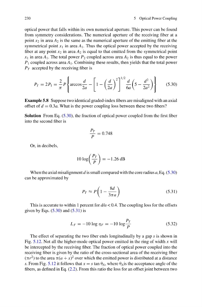
230
5 Optical Power Coupling
optical power that falls within its own numerical aperture. This power can be found
from symmetry considerations. The numerical aperture of the receiving fiber at a
point x 2 in area A 2 is the same as the numerical aperture of the emitting fiber at the
symmetrical point x 1 in area A 1 . Thus the optical power accepted by the receiving
fiber at any point x 2 in area A 2 is equal to that emitted from the symmetrical point
x 1 in area A 1 . The total power P 2 coupled across area A 2 is thus equal to the power
P 1 coupled across area A 1 . Combining these results, then yields that the total power
P T accepted by the receiving fiber is
P T = 2P 1 =
2
π
P
⎧
⎨
⎩
arccos
d
2a
−
1 −
d
2a
2
1/2
d
6a
5 −
d
2
2a 2
⎫
⎬
⎭
(5.30)
Example 5.8 Suppose two identical graded-index fibers are misaligned with an axial
offset of d = 0.3a. What is the power coupling loss between these two fibers?
Solution From Eq. (5.30), the fraction of optical power coupled from the first fiber
into the second fiber is
P T
P
= 0.748
Or, in decibels,
10 log
P T
P
= −1.26 dB
When the axial misalignment d is small compared with the core radius a, Eq. (5.30)
can be approximated by
P T ≈ P
1 −
8d
3πa
(5.31)
This is accurate to within 1 percent for d/a < 0.4. The coupling loss for the offsets
given by Eqs. (5.30) and (5.31) is
L F = −10 log η F = −10 log
P T
P
(5.32)
The effect of separating the two fiber ends longitudinally by a gap s is shown in
Fig. 5.12. Not all the higher-mode optical power emitted in the ring of width x will
be intercepted by the receiving fiber. The fraction of optical power coupled into the
receiving fiber is given by the ratio of the cross-sectional area of the receiving fiber
(πr
2 ) to the area π(a + x)
2 over which the emitted power is distributed at a distance
s. From Fig. 5.12 it follows that x = s tan θ A , where θ A is the acceptance angle of the
fibers, as defined in Eq. (2.2). From this ratio the loss for an offset joint between two
5 Optical Power Coupling
optical power that falls within its own numerical aperture. This power can be found
from symmetry considerations. The numerical aperture of the receiving fiber at a
point x 2 in area A 2 is the same as the numerical aperture of the emitting fiber at the
symmetrical point x 1 in area A 1 . Thus the optical power accepted by the receiving
fiber at any point x 2 in area A 2 is equal to that emitted from the symmetrical point
x 1 in area A 1 . The total power P 2 coupled across area A 2 is thus equal to the power
P 1 coupled across area A 1 . Combining these results, then yields that the total power
P T accepted by the receiving fiber is
P T = 2P 1 =
2
π
P
⎧
⎨
⎩
arccos
d
2a
−
1 −
d
2a
2
1/2
d
6a
5 −
d
2
2a 2
⎫
⎬
⎭
(5.30)
Example 5.8 Suppose two identical graded-index fibers are misaligned with an axial
offset of d = 0.3a. What is the power coupling loss between these two fibers?
Solution From Eq. (5.30), the fraction of optical power coupled from the first fiber
into the second fiber is
P T
P
= 0.748
Or, in decibels,
10 log
P T
P
= −1.26 dB
When the axial misalignment d is small compared with the core radius a, Eq. (5.30)
can be approximated by
P T ≈ P
1 −
8d
3πa
(5.31)
This is accurate to within 1 percent for d/a < 0.4. The coupling loss for the offsets
given by Eqs. (5.30) and (5.31) is
L F = −10 log η F = −10 log
P T
P
(5.32)
The effect of separating the two fiber ends longitudinally by a gap s is shown in
Fig. 5.12. Not all the higher-mode optical power emitted in the ring of width x will
be intercepted by the receiving fiber. The fraction of optical power coupled into the
receiving fiber is given by the ratio of the cross-sectional area of the receiving fiber
(πr
2 ) to the area π(a + x)
2 over which the emitted power is distributed at a distance
s. From Fig. 5.12 it follows that x = s tan θ A , where θ A is the acceptance angle of the
fibers, as defined in Eq. (2.2). From this ratio the loss for an offset joint between two