

5.3 Losses Between Fiber Joints
229
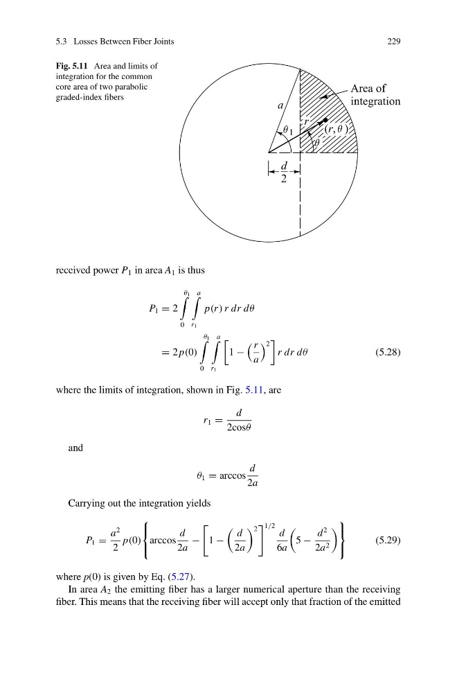
Fig. 5.11 Area and limits of
integration for the common
core area of two parabolic
graded-index fibers
received power P 1 in area A 1 is thus
P 1 = 2
θ 1
0
a
r 1
p(r ) r dr dθ
= 2 p(0)
θ 1
0
a
r 1
1 −
r
a
2
r dr dθ
(5.28)
where the limits of integration, shown in Fig. 5.11, are
r 1 =
d
2cosθ
and
θ 1 = arccos
d
2a
Carrying out the integration yields
P 1 =
a
2
2
p(0)
⎧
⎨
⎩
arccos
d
2a
−
1 −
d
2a
2
1/2
d
6a
5 −
d
2
2a 2
⎫
⎬
⎭
(5.29)
where p(0) is given by Eq. (5.27).
In area A 2 the emitting fiber has a larger numerical aperture than the receiving
fiber. This means that the receiving fiber will accept only that fraction of the emitted
229
Fig. 5.11 Area and limits of
integration for the common
core area of two parabolic
graded-index fibers
received power P 1 in area A 1 is thus
P 1 = 2
θ 1
0
a
r 1
p(r ) r dr dθ
= 2 p(0)
θ 1
0
a
r 1
1 −
r
a
2
r dr dθ
(5.28)
where the limits of integration, shown in Fig. 5.11, are
r 1 =
d
2cosθ
and
θ 1 = arccos
d
2a
Carrying out the integration yields
P 1 =
a
2
2
p(0)
⎧
⎨
⎩
arccos
d
2a
−
1 −
d
2a
2
1/2
d
6a
5 −
d
2
2a 2
⎫
⎬
⎭
(5.29)
where p(0) is given by Eq. (5.27).
In area A 2 the emitting fiber has a larger numerical aperture than the receiving
fiber. This means that the receiving fiber will accept only that fraction of the emitted