

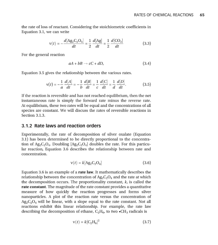
the rate of loss of reactant. Considering the stoichiometric coefficients in
Equation 3.1, we can write
n t
ð Þ = −
d Ag 2 C 2 O 4
½
dt
=
1
2
d Ag
½
dt
=
1
2
d CO 2
½
dt
(3.3)
For the general reaction
aA + bB ! cC + dD,
(3.4)
Equation 3.5 gives the relationship between the various rates.
v(t) = −
1
a
d A
½
dt
= −
1
b
d B
½
dt
=
1
c
d C
½
dt
=
1
d
d D
½
dt
:
(3.5)
If the reaction is reversible and has not reached equilibrium, then the net
instantaneous rate is simply the forward rate minus the reverse rate.
At equilibrium, these two rates will be equal and the concentrations of all
species are constant. We will discuss the rates of reversible reactions in
Section 3.1.3.
3.1.2 Rate laws and reaction orders
Experimentally, the rate of decomposition of silver oxalate (Equation
3.1) has been determined to be directly proportional to the concentration of Ag 2 C 2 O 4 . Doubling [Ag 2 C 2 O 4 ] doubles the rate. For this particular reaction, Equation 3.6 describes the relationship between rate and
concentration.
n t
ð Þ = k Ag 2 C 2 O 4
½
(3.6)
Equation 3.6 is an example of a rate law. It mathematically describes the
relationship between the concentration of Ag 2 C 2 O 4 and the rate at which
the decomposition occurs. The proportionality constant, k, is called the
rate constant. The magnitude of the rate constant provides a quantitative
measure of how quickly the reaction progresses and forms silver
nanoparticles. A plot of the reaction rate versus the concentration of
Ag 2 C 2 O 4 will be linear, with a slope equal to the rate constant. Not all
reactions exhibit this linear relationship. For example, the rate law
describing the decomposition of ethane, C 2 H 6 , to two •CH 3 radicals is
n t
ð Þ = k C 2 H 6
½
2
(3.7)
RATES OF CHEMICAL REACTIONS
65
Equation 3.1, we can write
n t
ð Þ = −
d Ag 2 C 2 O 4
½
dt
=
1
2
d Ag
½
dt
=
1
2
d CO 2
½
dt
(3.3)
For the general reaction
aA + bB ! cC + dD,
(3.4)
Equation 3.5 gives the relationship between the various rates.
v(t) = −
1
a
d A
½
dt
= −
1
b
d B
½
dt
=
1
c
d C
½
dt
=
1
d
d D
½
dt
:
(3.5)
If the reaction is reversible and has not reached equilibrium, then the net
instantaneous rate is simply the forward rate minus the reverse rate.
At equilibrium, these two rates will be equal and the concentrations of all
species are constant. We will discuss the rates of reversible reactions in
Section 3.1.3.
3.1.2 Rate laws and reaction orders
Experimentally, the rate of decomposition of silver oxalate (Equation
3.1) has been determined to be directly proportional to the concentration of Ag 2 C 2 O 4 . Doubling [Ag 2 C 2 O 4 ] doubles the rate. For this particular reaction, Equation 3.6 describes the relationship between rate and
concentration.
n t
ð Þ = k Ag 2 C 2 O 4
½
(3.6)
Equation 3.6 is an example of a rate law. It mathematically describes the
relationship between the concentration of Ag 2 C 2 O 4 and the rate at which
the decomposition occurs. The proportionality constant, k, is called the
rate constant. The magnitude of the rate constant provides a quantitative
measure of how quickly the reaction progresses and forms silver
nanoparticles. A plot of the reaction rate versus the concentration of
Ag 2 C 2 O 4 will be linear, with a slope equal to the rate constant. Not all
reactions exhibit this linear relationship. For example, the rate law
describing the decomposition of ethane, C 2 H 6 , to two •CH 3 radicals is
n t
ð Þ = k C 2 H 6
½
2
(3.7)
RATES OF CHEMICAL REACTIONS
65