

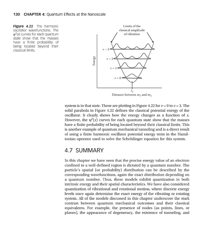
system is in that state. These are plotting in Figure 4.22 for v = 0 to v = 3. The
solid parabola in Figure 4.22 defines the classical potential energy of the
oscillator. It clearly shows how the energy changes as a function of x.
However, the y
2
(x) curves for each quantum state show that the masses
have a finite probability of being located beyond their classical limits. This
is another example of quantum mechanical tunneling and is a direct result
of using a finite harmonic oscillator potential energy term in the Hamiltonian operator used to solve the Schrödinger equation for this system.
4.7 SUMMARY
In this chapter we have seen that the precise energy value of an electron
confined to a well-defined region is dictated by a quantum number. The
particle’s spatial (or probability) distribution can be described by the
corresponding wavefunctions, again the exact distribution depending on
a quantum number. Thus, these models exhibit quantization in both
intrinsic energy and their spatial characteristics. We have also considered
quantization of vibrational and rotational motion, where discrete energy
levels once again determine the exact energy of the vibrating or rotating
system. All of the models discussed in this chapter underscore the stark
contrast between quantum mechanical outcomes and their classical
equivalents. For example, the presence of nodes (as points, lines, or
planes), the appearance of degeneracy, the existence of tunneling, and
Energy
Limits of the
classical amplitude
of vibration
v = 3
v = 2
v = 1
v = 0
Distance between m 1 and m 2
r e
Figure 4.22 The harmonic
oscillator wavefunctions. The
ψ
2
(x) curves for each quantum
state show that the masses
have a finite probability of
being located beyond their
classical limits.
CHAPTER 4: Quantum Effects at the Nanoscale
130
solid parabola in Figure 4.22 defines the classical potential energy of the
oscillator. It clearly shows how the energy changes as a function of x.
However, the y
2
(x) curves for each quantum state show that the masses
have a finite probability of being located beyond their classical limits. This
is another example of quantum mechanical tunneling and is a direct result
of using a finite harmonic oscillator potential energy term in the Hamiltonian operator used to solve the Schrödinger equation for this system.
4.7 SUMMARY
In this chapter we have seen that the precise energy value of an electron
confined to a well-defined region is dictated by a quantum number. The
particle’s spatial (or probability) distribution can be described by the
corresponding wavefunctions, again the exact distribution depending on
a quantum number. Thus, these models exhibit quantization in both
intrinsic energy and their spatial characteristics. We have also considered
quantization of vibrational and rotational motion, where discrete energy
levels once again determine the exact energy of the vibrating or rotating
system. All of the models discussed in this chapter underscore the stark
contrast between quantum mechanical outcomes and their classical
equivalents. For example, the presence of nodes (as points, lines, or
planes), the appearance of degeneracy, the existence of tunneling, and
Energy
Limits of the
classical amplitude
of vibration
v = 3
v = 2
v = 1
v = 0
Distance between m 1 and m 2
r e
Figure 4.22 The harmonic
oscillator wavefunctions. The
ψ
2
(x) curves for each quantum
state show that the masses
have a finite probability of
being located beyond their
classical limits.
CHAPTER 4: Quantum Effects at the Nanoscale
130