

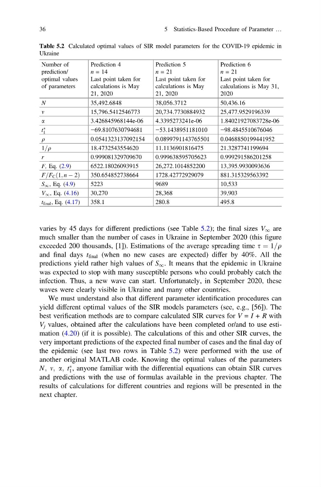
varies by 45 days for different predictions (see Table 5.2); the final sizes V 1 are
much smaller than the number of cases in Ukraine in September 2020 (this figure
exceeded 200 thousands, [1]). Estimations of the average spreading time s ¼ 1=q
and final days t final (when no new cases are expected) differ by 40%. All the
predictions yield rather high values of S 1 . It means that the epidemic in Ukraine
was expected to stop with many susceptible persons who could probably catch the
infection. Thus, a new wave can start. Unfortunately, in September 2020, these
waves were clearly visible in Ukraine and many other countries.
We must understand also that different parameter identification procedures can
yield different optimal values of the SIR models parameters (see, e.g., [56]). The
best verification methods are to compare calculated SIR curves for V = I + R with
V j values, obtained after the calculations have been completed or/and to use estimation (4.20) (if it is possible). The calculations of this and other SIR curves, the
very important predictions of the expected final number of cases and the final day of
the epidemic (see last two rows in Table 5.2) were performed with the use of
another original MATLAB code. Knowing the optimal values of the parameters
N; m; a; t
Ã
1 , anyone familiar with the differential equations can obtain SIR curves
and predictions with the use of formulas available in the previous chapter. The
results of calculations for different countries and regions will be presented in the
next chapter.
Table 5.2 Calculated optimal values of SIR model parameters for the COVID-19 epidemic in
Ukraine
Number of
prediction/
optimal values
of parameters
Prediction 4
n = 14
Last point taken for
calculations is May
21, 2020
Prediction 5
n = 21
Last point taken for
calculations is May
21, 2020
Prediction 6
n = 21
Last point taken for
calculations is May 31,
2020
N
35,492.6848
38,056.3712
50,436.16
m
15,796.5412546773
20,734.7730884932
25,477.9529196339
a
3.426845968144e-06
4.3395273241e-06
1.84021927083728e-06
t
Ã
1
−69.8107630794681
−53.1438951181010
−98.4845510676046
q
0.0541323137092154
0.0899791143765501
0.0468850199441952
1=q
18.4732543554620
11.1136901816475
21.3287741199694
r
0.999081329709670
0.999638595705623
0.999291586201258
F, Eq. (2.9)
6522.18026093915
26,272.1014852200
13,395.9930093636
F=F C 1; n À 2
ð
Þ
350.654852738664
1728.42772929079
881.315329563392
S 1 , Eq. (4.9)
5223
9689
10,533
V 1 , Eq. (4.16)
30,270
28,368
39,903
t final , Eq. (4.17)
358.1
280.8
495.8
36
5 Statistics-Based Procedure of Parameter …
much smaller than the number of cases in Ukraine in September 2020 (this figure
exceeded 200 thousands, [1]). Estimations of the average spreading time s ¼ 1=q
and final days t final (when no new cases are expected) differ by 40%. All the
predictions yield rather high values of S 1 . It means that the epidemic in Ukraine
was expected to stop with many susceptible persons who could probably catch the
infection. Thus, a new wave can start. Unfortunately, in September 2020, these
waves were clearly visible in Ukraine and many other countries.
We must understand also that different parameter identification procedures can
yield different optimal values of the SIR models parameters (see, e.g., [56]). The
best verification methods are to compare calculated SIR curves for V = I + R with
V j values, obtained after the calculations have been completed or/and to use estimation (4.20) (if it is possible). The calculations of this and other SIR curves, the
very important predictions of the expected final number of cases and the final day of
the epidemic (see last two rows in Table 5.2) were performed with the use of
another original MATLAB code. Knowing the optimal values of the parameters
N; m; a; t
Ã
1 , anyone familiar with the differential equations can obtain SIR curves
and predictions with the use of formulas available in the previous chapter. The
results of calculations for different countries and regions will be presented in the
next chapter.
Table 5.2 Calculated optimal values of SIR model parameters for the COVID-19 epidemic in
Ukraine
Number of
prediction/
optimal values
of parameters
Prediction 4
n = 14
Last point taken for
calculations is May
21, 2020
Prediction 5
n = 21
Last point taken for
calculations is May
21, 2020
Prediction 6
n = 21
Last point taken for
calculations is May 31,
2020
N
35,492.6848
38,056.3712
50,436.16
m
15,796.5412546773
20,734.7730884932
25,477.9529196339
a
3.426845968144e-06
4.3395273241e-06
1.84021927083728e-06
t
Ã
1
−69.8107630794681
−53.1438951181010
−98.4845510676046
q
0.0541323137092154
0.0899791143765501
0.0468850199441952
1=q
18.4732543554620
11.1136901816475
21.3287741199694
r
0.999081329709670
0.999638595705623
0.999291586201258
F, Eq. (2.9)
6522.18026093915
26,272.1014852200
13,395.9930093636
F=F C 1; n À 2
ð
Þ
350.654852738664
1728.42772929079
881.315329563392
S 1 , Eq. (4.9)
5223
9689
10,533
V 1 , Eq. (4.16)
30,270
28,368
39,903
t final , Eq. (4.17)
358.1
280.8
495.8
36
5 Statistics-Based Procedure of Parameter …