

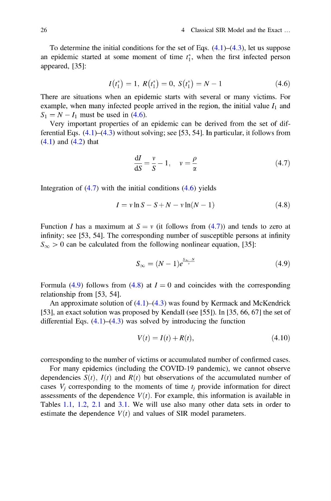
To determine the initial conditions for the set of Eqs. (4.1)–(4.3), let us suppose
an epidemic started at some moment of time t
Ã
1 , when the first infected person
appeared, [35]:
I t
Ã
1
À Á ¼ 1; R t
Ã
1
À Á ¼ 0; S t
Ã
1
À Á ¼ N À 1
ð4:6Þ
There are situations when an epidemic starts with several or many victims. For
example, when many infected people arrived in the region, the initial value I 1 and
S 1 ¼ N À I 1 must be used in (4.6).
Very important properties of an epidemic can be derived from the set of differential Eqs. (4.1)–(4.3) without solving; see [53, 54]. In particular, it follows from
(4.1) and (4.2) that
dI
dS
¼
m
S
À 1; m ¼
q
a
ð4:7Þ
Integration of (4.7) with the initial conditions (4.6) yields
I ¼ m ln S À S þ N À m lnðN À 1Þ
ð 4:8Þ
Function I has a maximum at S ¼ m (it follows from (4.7)) and tends to zero at
infinity; see [53, 54]. The corresponding number of susceptible persons at infinity
S 1 [ 0 can be calculated from the following nonlinear equation, [35]:
S 1 ¼ ðN À 1Þe
S1 ÀN
m
ð4:9Þ
Formula (4.9) follows from (4.8) at I ¼ 0 and coincides with the corresponding
relationship from [53, 54].
An approximate solution of (4.1)–(4.3) was found by Kermack and McKendrick
[53], an exact solution was proposed by Kendall (see [55]). In [35, 66, 67] the set of
differential Eqs. (4.1)–(4.3) was solved by introducing the function
VðtÞ ¼ IðtÞ þ RðtÞ;
ð4:10Þ
corresponding to the number of victims or accumulated number of confirmed cases.
For many epidemics (including the COVID-19 pandemic), we cannot observe
dependencies SðtÞ; IðtÞ and RðtÞ but observations of the accumulated number of
cases V j corresponding to the moments of time t j provide information for direct
assessments of the dependence VðtÞ. For example, this information is available in
Tables 1.1, 1.2, 2.1 and 3.1. We will use also many other data sets in order to
estimate the dependence VðtÞ and values of SIR model parameters.
26
4 Classical SIR Model and the Exact …
an epidemic started at some moment of time t
Ã
1 , when the first infected person
appeared, [35]:
I t
Ã
1
À Á ¼ 1; R t
Ã
1
À Á ¼ 0; S t
Ã
1
À Á ¼ N À 1
ð4:6Þ
There are situations when an epidemic starts with several or many victims. For
example, when many infected people arrived in the region, the initial value I 1 and
S 1 ¼ N À I 1 must be used in (4.6).
Very important properties of an epidemic can be derived from the set of differential Eqs. (4.1)–(4.3) without solving; see [53, 54]. In particular, it follows from
(4.1) and (4.2) that
dI
dS
¼
m
S
À 1; m ¼
q
a
ð4:7Þ
Integration of (4.7) with the initial conditions (4.6) yields
I ¼ m ln S À S þ N À m lnðN À 1Þ
ð 4:8Þ
Function I has a maximum at S ¼ m (it follows from (4.7)) and tends to zero at
infinity; see [53, 54]. The corresponding number of susceptible persons at infinity
S 1 [ 0 can be calculated from the following nonlinear equation, [35]:
S 1 ¼ ðN À 1Þe
S1 ÀN
m
ð4:9Þ
Formula (4.9) follows from (4.8) at I ¼ 0 and coincides with the corresponding
relationship from [53, 54].
An approximate solution of (4.1)–(4.3) was found by Kermack and McKendrick
[53], an exact solution was proposed by Kendall (see [55]). In [35, 66, 67] the set of
differential Eqs. (4.1)–(4.3) was solved by introducing the function
VðtÞ ¼ IðtÞ þ RðtÞ;
ð4:10Þ
corresponding to the number of victims or accumulated number of confirmed cases.
For many epidemics (including the COVID-19 pandemic), we cannot observe
dependencies SðtÞ; IðtÞ and RðtÞ but observations of the accumulated number of
cases V j corresponding to the moments of time t j provide information for direct
assessments of the dependence VðtÞ. For example, this information is available in
Tables 1.1, 1.2, 2.1 and 3.1. We will use also many other data sets in order to
estimate the dependence VðtÞ and values of SIR model parameters.
26
4 Classical SIR Model and the Exact …