

5.2 Critical State Model
83
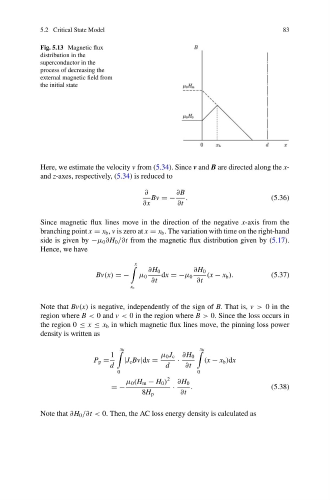
Fig. 5.13 Magnetic flux
distribution in the
superconductor in the
process of decreasing the
external magnetic field from
the initial state
Here, we estimate the velocity v from (5.34). Since v and B are directed along the xand z-axes, respectively, (5.34) is reduced to
∂
∂x
Bv = −
∂B
∂t
.
(5.36)
Since magnetic flux lines move in the direction of the negative x-axis from the
branching point x = x b , v is zero at x = x b . The variation with time on the right-hand
side is given by −μ 0 ∂H 0 /∂t from the magnetic flux distribution given by (5.17).
Hence, we have
Bv(x) = −
x
x b
μ 0
∂H 0
∂t
dx = −μ 0
∂H 0
∂t
(x − x b ).
(5.37)
Note that Bv(x) is negative, independently of the sign of B. That is, v > 0 in the
region where B < 0 and v < 0 in the region where B > 0. Since the loss occurs in
the region 0 ≤ x ≤ x b in which magnetic flux lines move, the pinning loss power
density is written as
P p =
1
d
x b
0
|J c Bv|dx =
μ 0 J c
d
·
∂H 0
∂t
x b
0
(x − x b )dx
= −
μ 0 (H m − H 0 )
2
8H p
·
∂H 0
∂t
.
(5.38)
Note that ∂H 0 /∂t < 0. Then, the AC loss energy density is calculated as
83
Fig. 5.13 Magnetic flux
distribution in the
superconductor in the
process of decreasing the
external magnetic field from
the initial state
Here, we estimate the velocity v from (5.34). Since v and B are directed along the xand z-axes, respectively, (5.34) is reduced to
∂
∂x
Bv = −
∂B
∂t
.
(5.36)
Since magnetic flux lines move in the direction of the negative x-axis from the
branching point x = x b , v is zero at x = x b . The variation with time on the right-hand
side is given by −μ 0 ∂H 0 /∂t from the magnetic flux distribution given by (5.17).
Hence, we have
Bv(x) = −
x
x b
μ 0
∂H 0
∂t
dx = −μ 0
∂H 0
∂t
(x − x b ).
(5.37)
Note that Bv(x) is negative, independently of the sign of B. That is, v > 0 in the
region where B < 0 and v < 0 in the region where B > 0. Since the loss occurs in
the region 0 ≤ x ≤ x b in which magnetic flux lines move, the pinning loss power
density is written as
P p =
1
d
x b
0
|J c Bv|dx =
μ 0 J c
d
·
∂H 0
∂t
x b
0
(x − x b )dx
= −
μ 0 (H m − H 0 )
2
8H p
·
∂H 0
∂t
.
(5.38)
Note that ∂H 0 /∂t < 0. Then, the AC loss energy density is calculated as