

58
4 Fundamental Electromagnetic Properties of Superconductors
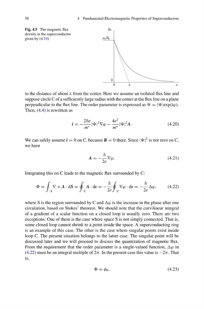
Fig. 4.5 The magnetic flux
density in the superconductor
given by (4.19)
to the distance of about λ from the center. Here we assume an isolated flux line and
suppose circle C of a sufficiently large radius with the center at the flux line on a plane
perpendicular to the flux line. The order parameter is expressed as = ||exp(iϕ).
Then, (4.4) is rewritten as
i = −
2e
m ∗ ||
2
∇ϕ −
4e
2
m ∗ ||
2 A.
(4.20)
We can safely assume i = 0 on C, because B = 0 there. Since ||
2 is not zero on C,
we have
A = −
2e
∇ϕ.
(4.21)
Integrating this on C leads to the magnetic flux surrounded by C:
=
S
∇ × A · dS =
C
A · ds = −
2e
C
∇ϕ · ds = −
2e
(4.22)
where S is the region surrounded by C and ϕ is the increase in the phase after one
circulation, based on Stokes’ theorem. We should note that the curvilinear integral
of a gradient of a scalar function on a closed loop is usually zero. There are two
exceptions: One of them is the case where space S is not simply connected. That is,
some closed loop cannot shrink to a point inside the space. A superconducting ring
is an example of this case. The other is the case where singular points exist inside
loop C. The present situation belongs to the latter case. The singular point will be
discussed later and we will proceed to discuss the quantization of magnetic flux.
From the requirement that the order parameter is a single-valued function, ϕ in
(4.22) must be an integral multiple of 2π . In the present case this value is −2π . That
is,
= φ 0 ,
(4.23)
4 Fundamental Electromagnetic Properties of Superconductors
Fig. 4.5 The magnetic flux
density in the superconductor
given by (4.19)
to the distance of about λ from the center. Here we assume an isolated flux line and
suppose circle C of a sufficiently large radius with the center at the flux line on a plane
perpendicular to the flux line. The order parameter is expressed as = ||exp(iϕ).
Then, (4.4) is rewritten as
i = −
2e
m ∗ ||
2
∇ϕ −
4e
2
m ∗ ||
2 A.
(4.20)
We can safely assume i = 0 on C, because B = 0 there. Since ||
2 is not zero on C,
we have
A = −
2e
∇ϕ.
(4.21)
Integrating this on C leads to the magnetic flux surrounded by C:
=
S
∇ × A · dS =
C
A · ds = −
2e
C
∇ϕ · ds = −
2e
(4.22)
where S is the region surrounded by C and ϕ is the increase in the phase after one
circulation, based on Stokes’ theorem. We should note that the curvilinear integral
of a gradient of a scalar function on a closed loop is usually zero. There are two
exceptions: One of them is the case where space S is not simply connected. That is,
some closed loop cannot shrink to a point inside the space. A superconducting ring
is an example of this case. The other is the case where singular points exist inside
loop C. The present situation belongs to the latter case. The singular point will be
discussed later and we will proceed to discuss the quantization of magnetic flux.
From the requirement that the order parameter is a single-valued function, ϕ in
(4.22) must be an integral multiple of 2π . In the present case this value is −2π . That
is,
= φ 0 ,
(4.23)