

3.1 Electricity in a Conductor and Magnetism in a Superconductor
35
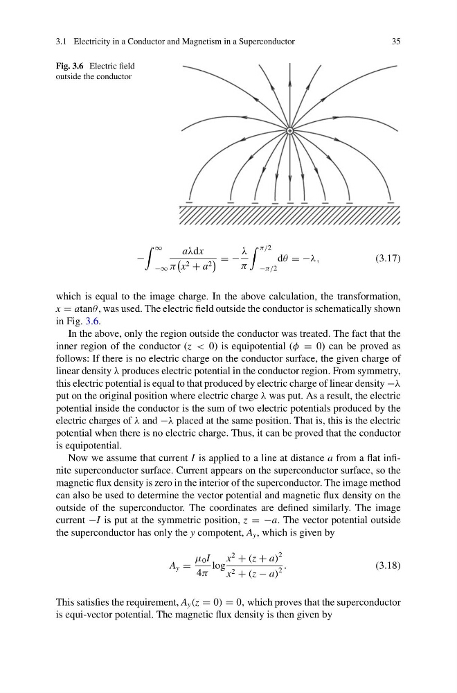
Fig. 3.6 Electric field
outside the conductor
−
∞
−∞
aλdx
π
x 2 + a 2
= −
λ
π
π/2
−π/2
dθ = −λ,
(3.17)
which is equal to the image charge. In the above calculation, the transformation,
x = atanθ , was used. The electric field outside the conductor is schematically shown
in Fig. 3.6.
In the above, only the region outside the conductor was treated. The fact that the
inner region of the conductor (z < 0) is equipotential (φ = 0) can be proved as
follows: If there is no electric charge on the conductor surface, the given charge of
linear density λ produces electric potential in the conductor region. From symmetry,
this electric potential is equal to that produced by electric charge of linear density −λ
put on the original position where electric charge λ was put. As a result, the electric
potential inside the conductor is the sum of two electric potentials produced by the
electric charges of λ and −λ placed at the same position. That is, this is the electric
potential when there is no electric charge. Thus, it can be proved that the conductor
is equipotential.
Now we assume that current I is applied to a line at distance a from a flat infinite superconductor surface. Current appears on the superconductor surface, so the
magnetic flux density is zero in the interior of the superconductor. The image method
can also be used to determine the vector potential and magnetic flux density on the
outside of the superconductor. The coordinates are defined similarly. The image
current −I is put at the symmetric position, z = −a. The vector potential outside
the superconductor has only the y compotent, A y , which is given by
A y =
μ 0 I
4π
log
x
2
+ (z + a)
2
x 2 + (z − a)
2
.
(3.18)
This satisfies the requirement, A y (z = 0) = 0, which proves that the superconductor
is equi-vector potential. The magnetic flux density is then given by
35
Fig. 3.6 Electric field
outside the conductor
−
∞
−∞
aλdx
π
x 2 + a 2
= −
λ
π
π/2
−π/2
dθ = −λ,
(3.17)
which is equal to the image charge. In the above calculation, the transformation,
x = atanθ , was used. The electric field outside the conductor is schematically shown
in Fig. 3.6.
In the above, only the region outside the conductor was treated. The fact that the
inner region of the conductor (z < 0) is equipotential (φ = 0) can be proved as
follows: If there is no electric charge on the conductor surface, the given charge of
linear density λ produces electric potential in the conductor region. From symmetry,
this electric potential is equal to that produced by electric charge of linear density −λ
put on the original position where electric charge λ was put. As a result, the electric
potential inside the conductor is the sum of two electric potentials produced by the
electric charges of λ and −λ placed at the same position. That is, this is the electric
potential when there is no electric charge. Thus, it can be proved that the conductor
is equipotential.
Now we assume that current I is applied to a line at distance a from a flat infinite superconductor surface. Current appears on the superconductor surface, so the
magnetic flux density is zero in the interior of the superconductor. The image method
can also be used to determine the vector potential and magnetic flux density on the
outside of the superconductor. The coordinates are defined similarly. The image
current −I is put at the symmetric position, z = −a. The vector potential outside
the superconductor has only the y compotent, A y , which is given by
A y =
μ 0 I
4π
log
x
2
+ (z + a)
2
x 2 + (z − a)
2
.
(3.18)
This satisfies the requirement, A y (z = 0) = 0, which proves that the superconductor
is equi-vector potential. The magnetic flux density is then given by