

2.2 Static Magnetic Phenomena
19
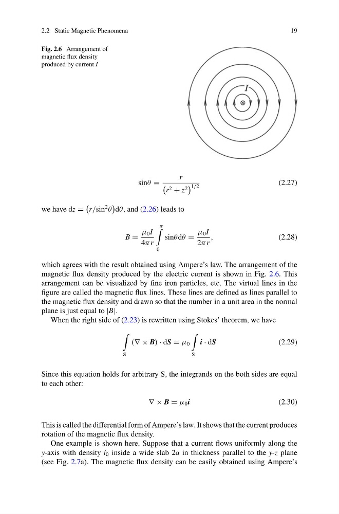
Fig. 2.6 Arrangement of
magnetic flux density
produced by current I
sinθ =
r
r 2 + z 2
1/2
(2.27)
we have dz =
r/sin
2
θ
dθ , and (2.26) leads to
B =
μ 0 I
4π r
π
0
sinθ dθ =
μ 0 I
2π r
,
(2.28)
which agrees with the result obtained using Ampere’s law. The arrangement of the
magnetic flux density produced by the electric current is shown in Fig. 2.6. This
arrangement can be visualized by fine iron particles, etc. The virtual lines in the
figure are called the magnetic flux lines. These lines are defined as lines parallel to
the magnetic flux density and drawn so that the number in a unit area in the normal
plane is just equal to |B|.
When the right side of (2.23) is rewritten using Stokes’ theorem, we have
S
(∇ × B) · dS = μ 0
S
i · dS
(2.29)
Since this equation holds for arbitrary S, the integrands on the both sides are equal
to each other:
∇ × B = μ 0 i
(2.30)
This is called the differential form of Ampere’s law. It shows that the current produces
rotation of the magnetic flux density.
One example is shown here. Suppose that a current flows uniformly along the
y-axis with density i 0 inside a wide slab 2a in thickness parallel to the y-z plane
(see Fig. 2.7a). The magnetic flux density can be easily obtained using Ampere’s
19
Fig. 2.6 Arrangement of
magnetic flux density
produced by current I
sinθ =
r
r 2 + z 2
1/2
(2.27)
we have dz =
r/sin
2
θ
dθ , and (2.26) leads to
B =
μ 0 I
4π r
π
0
sinθ dθ =
μ 0 I
2π r
,
(2.28)
which agrees with the result obtained using Ampere’s law. The arrangement of the
magnetic flux density produced by the electric current is shown in Fig. 2.6. This
arrangement can be visualized by fine iron particles, etc. The virtual lines in the
figure are called the magnetic flux lines. These lines are defined as lines parallel to
the magnetic flux density and drawn so that the number in a unit area in the normal
plane is just equal to |B|.
When the right side of (2.23) is rewritten using Stokes’ theorem, we have
S
(∇ × B) · dS = μ 0
S
i · dS
(2.29)
Since this equation holds for arbitrary S, the integrands on the both sides are equal
to each other:
∇ × B = μ 0 i
(2.30)
This is called the differential form of Ampere’s law. It shows that the current produces
rotation of the magnetic flux density.
One example is shown here. Suppose that a current flows uniformly along the
y-axis with density i 0 inside a wide slab 2a in thickness parallel to the y-z plane
(see Fig. 2.7a). The magnetic flux density can be easily obtained using Ampere’s