

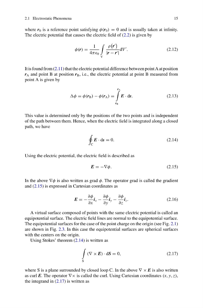
2.1 Electrostatic Phenomena
15
where r 0 is a reference point satisfying φ(r 0 ) = 0 and is usually taken at infinity.
The electric potential that causes the electric field of (2.2) is given by
φ(r) =
1
4ππ 0
V
ρ
r
|r − r |
dV
.
(2.12)
It is found from (2.11) that the electric potential difference between point A at position
r A and point B at position r B , i.e., the electric potential at point B measured from
point A is given by
φ = φ(r B ) − φ(r A ) =
r A
r B
E · ds.
(2.13)
This value is determined only by the positions of the two points and is independent
of the path between them. Hence, when the electric field is integrated along a closed
path, we have
C
E · ds = 0.
(2.14)
Using the electric potential, the electric field is described as
E = −∇φ.
(2.15)
In the above ∇φ is also written as grad φ. The operator grad is called the gradient
and (2.15) is expressed in Cartesian coordinates as
E = −
∂φ
∂x
i x −
∂φ
∂y
i y −
∂φ
∂z
i z .
(2.16)
A virtual surface composed of points with the same electric potential is called an
equipotential surface. The electric field lines are normal to the equipotential surface.
The equipotential surfaces for the case of the point charge on the origin (see Fig. 2.1)
are shown in Fig. 2.3. In this case the equipotential surfaces are spherical surfaces
with the centers on the origin.
Using Stokes’ theorem (2.14) is written as
S
(∇ × E) · dS = 0,
(2.17)
where S is a plane surrounded by closed loop C. In the above ∇ × E is also written
as curl E. The operator ∇× is called the curl. Using Cartesian coordinates (x, y, z),
the integrand in (2.17) is written as
15
where r 0 is a reference point satisfying φ(r 0 ) = 0 and is usually taken at infinity.
The electric potential that causes the electric field of (2.2) is given by
φ(r) =
1
4ππ 0
V
ρ
r
|r − r |
dV
.
(2.12)
It is found from (2.11) that the electric potential difference between point A at position
r A and point B at position r B , i.e., the electric potential at point B measured from
point A is given by
φ = φ(r B ) − φ(r A ) =
r A
r B
E · ds.
(2.13)
This value is determined only by the positions of the two points and is independent
of the path between them. Hence, when the electric field is integrated along a closed
path, we have
C
E · ds = 0.
(2.14)
Using the electric potential, the electric field is described as
E = −∇φ.
(2.15)
In the above ∇φ is also written as grad φ. The operator grad is called the gradient
and (2.15) is expressed in Cartesian coordinates as
E = −
∂φ
∂x
i x −
∂φ
∂y
i y −
∂φ
∂z
i z .
(2.16)
A virtual surface composed of points with the same electric potential is called an
equipotential surface. The electric field lines are normal to the equipotential surface.
The equipotential surfaces for the case of the point charge on the origin (see Fig. 2.1)
are shown in Fig. 2.3. In this case the equipotential surfaces are spherical surfaces
with the centers on the origin.
Using Stokes’ theorem (2.14) is written as
S
(∇ × E) · dS = 0,
(2.17)
where S is a plane surrounded by closed loop C. In the above ∇ × E is also written
as curl E. The operator ∇× is called the curl. Using Cartesian coordinates (x, y, z),
the integrand in (2.17) is written as