

138
6 Longitudinal Magnetic Field Effect
Finally, we discuss the phenomena in the resistive state. In the transverse magnetic
field, the Lorentz force exceeds the pinning force, and flux flow occurs. By analogy,
it is speculated that flux lines become unstable under a force-free torque that exceeds
the pinning torque. The expected motion of flux lines in this case is rotation driven
by the excess force-free torque. In this section an example of such a rotation was
shown in the quasi-static condition. This is the rotation illustrated in Fig. 6.11. In
the usual resistive state, however, if only such a rotation occurs, the steady condition
does not hold. To keep the steady state, when the flux lines in the former plane rotate
as shown by the arrows, those must move to the next plane, i.e., to the place of the
flux lines of the adjacent plane in the former instance. The steady state can be kept
under the rotational motion accompanied by such a translational motion. Since the
Lorentz force on the flux lines is zero, no energy dissipation occurs due to the induced
translational motion.
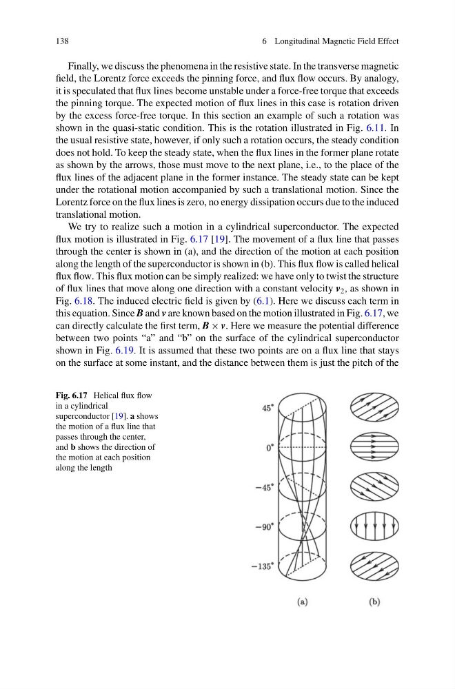
We try to realize such a motion in a cylindrical superconductor. The expected
flux motion is illustrated in Fig. 6.17 [19]. The movement of a flux line that passes
through the center is shown in (a), and the direction of the motion at each position
along the length of the superconductor is shown in (b). This flux flow is called helical
flux flow. This flux motion can be simply realized: we have only to twist the structure
of flux lines that move along one direction with a constant velocity v 2 , as shown in
Fig. 6.18. The induced electric field is given by (6.1). Here we discuss each term in
this equation. Since B and v are known based on the motion illustrated in Fig. 6.17, we
can directly calculate the first term, B × v. Here we measure the potential difference
between two points “a” and “b” on the surface of the cylindrical superconductor
shown in Fig. 6.19. It is assumed that these two points are on a flux line that stays
on the surface at some instant, and the distance between them is just the pitch of the
Fig. 6.17 Helical flux flow
in a cylindrical
superconductor [19]. a shows
the motion of a flux line that
passes through the center,
and b shows the direction of
the motion at each position
along the length
6 Longitudinal Magnetic Field Effect
Finally, we discuss the phenomena in the resistive state. In the transverse magnetic
field, the Lorentz force exceeds the pinning force, and flux flow occurs. By analogy,
it is speculated that flux lines become unstable under a force-free torque that exceeds
the pinning torque. The expected motion of flux lines in this case is rotation driven
by the excess force-free torque. In this section an example of such a rotation was
shown in the quasi-static condition. This is the rotation illustrated in Fig. 6.11. In
the usual resistive state, however, if only such a rotation occurs, the steady condition
does not hold. To keep the steady state, when the flux lines in the former plane rotate
as shown by the arrows, those must move to the next plane, i.e., to the place of the
flux lines of the adjacent plane in the former instance. The steady state can be kept
under the rotational motion accompanied by such a translational motion. Since the
Lorentz force on the flux lines is zero, no energy dissipation occurs due to the induced
translational motion.
We try to realize such a motion in a cylindrical superconductor. The expected
flux motion is illustrated in Fig. 6.17 [19]. The movement of a flux line that passes
through the center is shown in (a), and the direction of the motion at each position
along the length of the superconductor is shown in (b). This flux flow is called helical
flux flow. This flux motion can be simply realized: we have only to twist the structure
of flux lines that move along one direction with a constant velocity v 2 , as shown in
Fig. 6.18. The induced electric field is given by (6.1). Here we discuss each term in
this equation. Since B and v are known based on the motion illustrated in Fig. 6.17, we
can directly calculate the first term, B × v. Here we measure the potential difference
between two points “a” and “b” on the surface of the cylindrical superconductor
shown in Fig. 6.19. It is assumed that these two points are on a flux line that stays
on the surface at some instant, and the distance between them is just the pitch of the
Fig. 6.17 Helical flux flow
in a cylindrical
superconductor [19]. a shows
the motion of a flux line that
passes through the center,
and b shows the direction of
the motion at each position
along the length