

6.4 Electromagnetic Phenomena Caused by Rotation of Flux Lines
135
∂θ
∂t
= α f v y +
1
sinθ cosθ
·
∂v x
∂x
.
(6.42)
Here we assume a quasi-static process. That is, the variation with time comes only
through the variation in the self-field H I of the current. Then, the left-hand sides of
(6.41) and (6.42) are respectively given by
∂B
∂t
= μ 0 sinθ 0
∂H I
∂t
(6.43)
and
∂θ
∂t
=
∂θ 0
∂t
=
μ 0 cosθ 0
B
·
∂H I
∂t
.
(6.44)
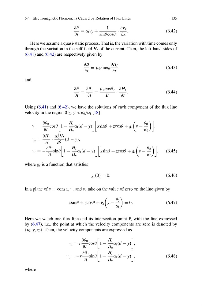
Using (6.41) and (6.42), we have the solutions of each component of the flux line
velocity in the region 0 ≤ y < θ 0 /α f [18]
v x =
∂θ 0
∂t
cosθ
1 −
H I
H e
α f (d − y)
xsinθ + zcosθ + g r
y −
θ 0
α f
,
v y =
∂H I
∂t
·
μ
2
0 H I
B 2 (d − y),
v z = −
∂θ 0
∂t
sinθ
1 −
H I
H e
α f (d − y)
xsinθ + zcosθ + g r
y −
θ 0
α f
,
(6.45)
where g r is a function that satisfies
g r (0) = 0.
(6.46)
In a plane of y = const., v x and v z take on the value of zero on the line given by
xsinθ + zcosθ + g r
y −
θ 0
α f
= 0.
(6.47)
Here we watch one flux line and its intersection point P, with the line expressed
by (6.47), i.e., the point at which the velocity components are zero is denoted by
(x 0 , y, z 0 ). Then, the velocity components are expressed as
v x = r
∂θ 0
∂t
cosθ
1 −
H I
H e
α f (d − y)
,
v z = −r
∂θ 0
∂t
sinθ
1 −
H I
H e
α f (d − y)
,
(6.48)
where
135
∂θ
∂t
= α f v y +
1
sinθ cosθ
·
∂v x
∂x
.
(6.42)
Here we assume a quasi-static process. That is, the variation with time comes only
through the variation in the self-field H I of the current. Then, the left-hand sides of
(6.41) and (6.42) are respectively given by
∂B
∂t
= μ 0 sinθ 0
∂H I
∂t
(6.43)
and
∂θ
∂t
=
∂θ 0
∂t
=
μ 0 cosθ 0
B
·
∂H I
∂t
.
(6.44)
Using (6.41) and (6.42), we have the solutions of each component of the flux line
velocity in the region 0 ≤ y < θ 0 /α f [18]
v x =
∂θ 0
∂t
cosθ
1 −
H I
H e
α f (d − y)
xsinθ + zcosθ + g r
y −
θ 0
α f
,
v y =
∂H I
∂t
·
μ
2
0 H I
B 2 (d − y),
v z = −
∂θ 0
∂t
sinθ
1 −
H I
H e
α f (d − y)
xsinθ + zcosθ + g r
y −
θ 0
α f
,
(6.45)
where g r is a function that satisfies
g r (0) = 0.
(6.46)
In a plane of y = const., v x and v z take on the value of zero on the line given by
xsinθ + zcosθ + g r
y −
θ 0
α f
= 0.
(6.47)
Here we watch one flux line and its intersection point P, with the line expressed
by (6.47), i.e., the point at which the velocity components are zero is denoted by
(x 0 , y, z 0 ). Then, the velocity components are expressed as
v x = r
∂θ 0
∂t
cosθ
1 −
H I
H e
α f (d − y)
,
v z = −r
∂θ 0
∂t
sinθ
1 −
H I
H e
α f (d − y)
,
(6.48)
where