

6.2 Clue to the Solution
127
J = −
B
μ 0
·
∂θ
∂y
.
(6.14)
Hence, the angle of flux lines is expressed as
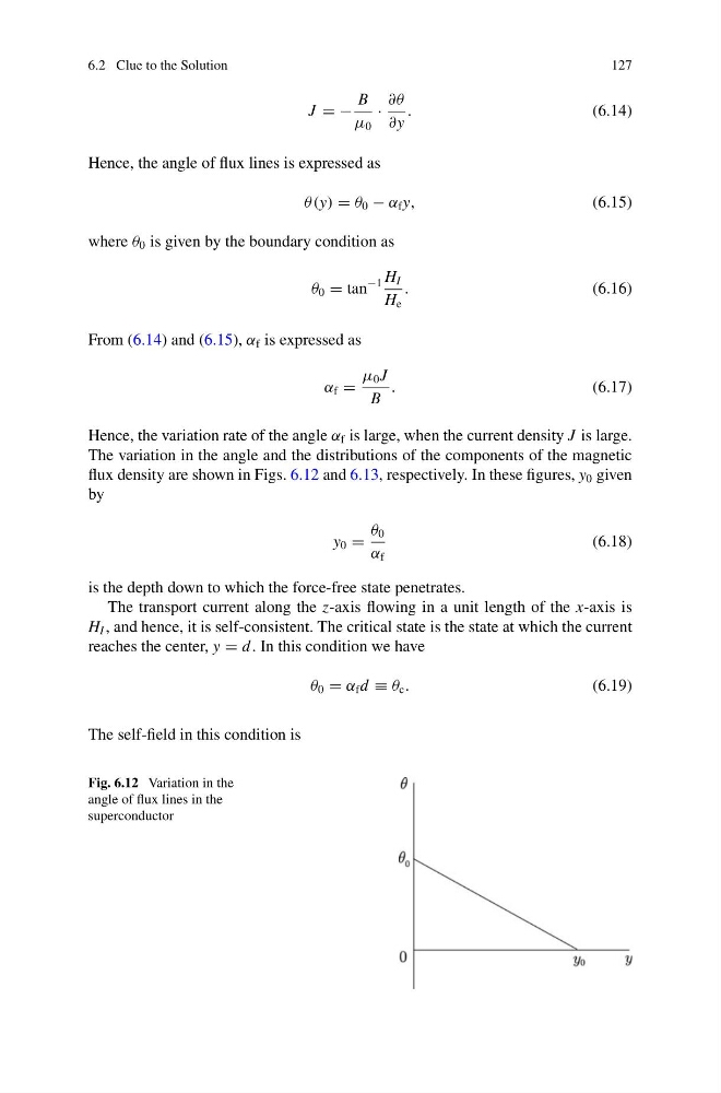
θ (y) = θ 0 − α f y,
(6.15)
where θ 0 is given by the boundary condition as
θ 0 = tan
−1 H I
H e
.
(6.16)
From (6.14) and (6.15), α f is expressed as
α f =
μ 0 J
B
.
(6.17)
Hence, the variation rate of the angle α f is large, when the current density J is large.
The variation in the angle and the distributions of the components of the magnetic
flux density are shown in Figs. 6.12 and 6.13, respectively. In these figures, y 0 given
by
y 0 =
θ 0
α f
(6.18)
is the depth down to which the force-free state penetrates.
The transport current along the z-axis flowing in a unit length of the x-axis is
H I , and hence, it is self-consistent. The critical state is the state at which the current
reaches the center, y = d . In this condition we have
θ 0 = α f d ≡ θ c .
(6.19)
The self-field in this condition is
Fig. 6.12 Variation in the
angle of flux lines in the
superconductor
127
J = −
B
μ 0
·
∂θ
∂y
.
(6.14)
Hence, the angle of flux lines is expressed as
θ (y) = θ 0 − α f y,
(6.15)
where θ 0 is given by the boundary condition as
θ 0 = tan
−1 H I
H e
.
(6.16)
From (6.14) and (6.15), α f is expressed as
α f =
μ 0 J
B
.
(6.17)
Hence, the variation rate of the angle α f is large, when the current density J is large.
The variation in the angle and the distributions of the components of the magnetic
flux density are shown in Figs. 6.12 and 6.13, respectively. In these figures, y 0 given
by
y 0 =
θ 0
α f
(6.18)
is the depth down to which the force-free state penetrates.
The transport current along the z-axis flowing in a unit length of the x-axis is
H I , and hence, it is self-consistent. The critical state is the state at which the current
reaches the center, y = d . In this condition we have
θ 0 = α f d ≡ θ c .
(6.19)
The self-field in this condition is
Fig. 6.12 Variation in the
angle of flux lines in the
superconductor